Decoding Immune Disease Networks: A Comprehensive Guide to GWAS and Genomic SEM for Researchers
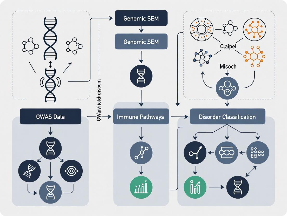
This article provides a detailed technical guide for researchers and drug development professionals on applying Genome-Wide Association Studies (GWAS) and Genomic Structural Equation Modeling (Genomic SEM) to classify and understand...
Decoding Immune Disease Networks: A Comprehensive Guide to GWAS and Genomic SEM for Researchers
Abstract
This article provides a detailed technical guide for researchers and drug development professionals on applying Genome-Wide Association Studies (GWAS) and Genomic Structural Equation Modeling (Genomic SEM) to classify and understand the shared genetic architecture of immune-mediated disorders. It covers foundational concepts, advanced methodological workflows, common troubleshooting strategies, and validation techniques. The content explores how these integrated approaches can disentangle pleiotropy, identify latent genetic factors, and inform the development of more targeted therapeutics by moving beyond traditional diagnostic categories to biologically defined disease subtypes.
The Genetic Landscape of Immune Disorders: From GWAS Hits to Shared Biology
Immune-mediated inflammatory diseases (IMIDs) such as rheumatoid arthritis (RA), inflammatory bowel disease (IBD), psoriasis (Ps), and multiple sclerosis (MS) represent a significant clinical and research challenge due to their overlapping clinical presentations and shared genetic architectures. This pleiotropy complicates diagnosis, obscures pathogenic mechanisms, and impacts therapeutic development. Within the context of advanced genomic research, Genome-Wide Association Studies (GWAS) have identified thousands of risk loci, but their biological interpretation remains limited. Genomic Structural Equation Modeling (SEM) emerges as a critical framework for disentangling shared and specific genetic factors across IMIDs, moving beyond single-disease analysis to a systems-level understanding.
Quantitative Data: Shared Heritability and Loci
Table 1: Genetic Correlation (rg) Between Selected Immune-Mediated Diseases (Recent Estimates)
| Disease Pair | Genetic Correlation (rg) | Standard Error | Primary Source |
|---|---|---|---|
| Rheumatoid Arthritis (RA) & Crohn's Disease (CD) | 0.33 | 0.03 | Cross-Disorder GWAS Meta-analysis (2023) |
| Ulcerative Colitis (UC) & Ankylosing Spondylitis (AS) | 0.28 | 0.04 | Cross-Disorder GWAS Meta-analysis (2023) |
| Psoriasis & Crohn's Disease (CD) | 0.45 | 0.04 | Cross-Disorder GWAS Meta-analysis (2023) |
| Multiple Sclerosis (MS) & Rheumatoid Arthritis (RA) | -0.05 | 0.04 | Cross-Disorder GWAS Meta-analysis (2023) |
Table 2: Top Pleiotropic Genomic Loci in IMIDs
| Locus (Nearest Gene) | Associated Diseases (p < 5e-08) | Proposed Functional Pathway |
|---|---|---|
| 6p21 (MHC Region) | RA, IBD, Ps, AS, MS, T1D | Antigen Presentation, Immune Activation |
| 1q32 (IL10, IL19, IL20) | UC, Ps, IBD | IL-10/IL-20 Family Signaling, Mucosal Immunity |
| 3p21 (CCR5, CCR3) | RA, MS, Ps, CD | Chemokine Signaling, Leukocyte Migration |
| 5q33 (IL12B) | Ps, CD, AS | Th1/Th17 Cell Differentiation |
Application Notes: Genomic SEM for IMID Classification
Objective: To partition aggregated SNP-level GWAS data into genetically independent but potentially correlated latent factors representing shared and disease-specific liabilities.
Pre-processing Workflow:
- Data Input: Obtain GWAS summary statistics (SNP, effect allele, non-effect allele, beta, SE, p-value, sample size) for at least 4-5 phenotypically overlapping IMIDs.
- Quality Control & Harmonization: Use tools like
MungeSumstatsto align alleles, filter on INFO score >0.9, and remove strand-ambiguous and duplicate SNPs. - LD Score Regression: Estimate genetic covariance and heritability matrices using LDSC (
--rgflag) to inform the initial model structure.
Model Specification: A common factor model can be tested where a latent "Broad Autoimmune" factor loads onto all diseases, and specific factors account for residual variance unique to subsets (e.g., a "Mucosal Immunity" factor loading on IBD and UC).
Experimental Protocols
Protocol 4.1: In Silico Fine-Mapping and Colocalization at Pleiotropic Loci
Objective: To identify candidate causal variants and assess if the same variant drives association signals across multiple IMIDs.
Materials & Reagents: GWAS summary statistics for ≥2 diseases; matched eQTL/sQTL data (e.g., from GTEx, DICE, BLUEPRINT); reference panel (1000 Genomes Phase 3 EUR); software: coloc, SuSiE, LocusCompareR.
Method:
- Define Locus Regions: For each pleiotropic locus from Table 2, extract a ±500 kb region around the lead SNP.
- Harmonize Datasets: Ensure all datasets (GWAS, QTL) use the same genome build and allele coding. Flip strands as necessary.
- Statistical Fine-mapping: For each disease GWAS in the region, run
SuSiEto generate a credible set of causal variants (e.g., 95% credible set). - Colocalization Analysis: Run
colocusing default priors (p1=1e-4, p2=1e-4, p12=1e-5) pairwise between diseases and between each disease and relevant QTL datasets. - Interpretation: A posterior probability for colocalization (PP.H4) > 0.8 suggests a shared causal variant. Overlap of credible sets provides supporting evidence.
Protocol 4.2: Functional Validation of Pleiotropic Variants using CRISPRi in Immune Cell Lines
Objective: To experimentally validate the regulatory function of a non-coding candidate causal variant on immune gene expression.
Materials & Reagents: THP-1 (monocyte) and/or Jurkat (T-cell) cell lines; Lentiviral vectors for dCas9-KRAB; sgRNA design and synthesis kits; Lipofectamine 3000; Puromycin; RNA extraction kit (e.g., RNeasy); qPCR reagents; primers for target gene.
Method:
- sgRNA Design: Design 2-3 sgRNAs targeting within 100bp of the candidate SNP for CRISPR interference (CRISPRi). Include a non-targeting control sgRNA.
- Stable Cell Line Generation: Co-transfect packaging cells with lentiviral dCas9-KRAB and sgRNA vectors. Harvest virus and transduce target immune cell lines. Select with puromycin (1-2 µg/mL) for 7 days.
- Stimulation: Differentiate/activate cells as needed (e.g., THP-1 with PMA/ionomycin; Jurkat with anti-CD3/CD28 beads).
- Phenotypic Readout: Harvest cells 48h post-stimulation. Extract RNA, synthesize cDNA, and perform qPCR for the putative target gene(s) identified by colocalization (e.g., IL12B).
- Analysis: Calculate ΔΔCt relative to non-targeting sgRNA control. Compare expression between sgRNAs targeting the risk vs. non-risk haplotype (if applicable). Statistical test: unpaired t-test.
Visualizations
Diagram 1: Genomic SEM Model for IMID Pleiotropy (76 chars)
Diagram 2: Colocalization & Validation Workflow (80 chars)
The Scientist's Toolkit: Research Reagent Solutions
Table 3: Essential Reagents and Resources for IMID Pleiotropy Research
| Item | Function/Application | Example Product/Resource |
|---|---|---|
| GWAS Summary Statistics | Foundational data for genetic correlation, SEM, and fine-mapping. | NHGRI-EBI GWAS Catalog; IBD Genetics, PGC, etc. |
| LDSC Software Suite | Estimates heritability and genetic correlation; critical for model building. | ldsc (python package) |
| Genomic SEM Software | Fits multivariate models to GWAS data to factorize genetic risk. | GenomicSEM (R package) |
| Colocalization Tool | Tests hypothesis of shared causal variant across traits/molecular QTLs. | coloc (R package) |
| Fine-mapping Tool | Refines association signals to credible sets of causal variants. | SuSiE, FINEMAP |
| Immune Cell eQTL Data | Links genetic variants to gene expression in relevant cell types. | DICE database, BLUEPRINT, GTEx |
| CRISPRi/a System | For perturbing non-coding risk variants in relevant cellular contexts. | dCas9-KRAB (for repression) lentiviral kits |
| Polarized Immune Cell Models | Functional assays in disease-relevant cell states (e.g., Th17, M1 macrophages). | Primary CD4+ T-cells, iPSC-derived macrophages, organoids |
This document serves as a foundational refresher on Genome-Wide Association Studies (GWAS) within the context of a doctoral thesis investigating the genetic architecture of immune-mediated disorders (IMDs) using GWAS and genomic Structural Equation Modeling (SEM). The integration of high-throughput GWAS data from public repositories with advanced statistical methods like genomic SEM is pivotal for moving beyond single-variant associations to model shared genetic factors and causal pathways across related IMDs, such as rheumatoid arthritis, Crohn's disease, and multiple sclerosis. This progression is essential for refined classification and identifying novel therapeutic targets.
Core Principles of GWAS
A GWAS is an observational study that tests for statistical associations between genetic variants (typically single nucleotide polymorphisms, SNPs) and a trait (e.g., disease status or quantitative biomarker) across the genome in a population. Its fundamental principle is the "common disease-common variant" hypothesis.
Key Design Considerations:
- Population & Sample Size: Large cohorts (often tens to hundreds of thousands) are required to achieve statistical power for variants with small effect sizes. Population stratification must be controlled.
- Genotyping & Imputation: Participants are genotyped using microarray chips covering 500K to 2M variants. Statistical imputation (e.g., with tools like IMPUTE4 or Minimac4) is then used to infer ungenotyped variants based on reference panels (e.g., 1000 Genomes, TOPMed), expanding the analyzed variant set to ~10-20 million.
- Phenotyping: Precise, consistent trait measurement is critical. For IMD research, this often involves clinical diagnostic criteria, biomarker levels (e.g., cytokine levels), or electronic health record data.
- Statistical Analysis: A generalized linear model tests each variant for association, typically adjusting for covariates like age, sex, and genetic principal components to control for confounding.
GWAS Outputs: Interpretation and Meaning
Primary Outputs Table
| Output | Description | Typical Range/Format | Interpretation in IMD Research |
|---|---|---|---|
| SNP Identifier (rsID) | Unique reference SNP cluster ID. | rs[number] (e.g., rs2476601) | Maps the association to a specific genomic location. For IMDs, may flag genes in immune pathways (e.g., PTPN22 rs2476601 in T-cell signaling). |
| Chromosome & Position | Genomic coordinates (build GRCh38). | chr[number]:[base pair position] | Identifies the locus for functional follow-up and colocalization with regulatory elements (e.g., enhancers in immune cells). |
| Effect Allele (EA) / Other Allele (OA) | The allele tested for effect size. OA is the reference/comparison. | A, T, C, G | The EA is the allele associated with the trait. The direction of effect is crucial for genomic SEM modeling of genetic correlations. |
| Effect Size (β / OR) | Magnitude and direction of the allele's effect. | β (continuous trait), Odds Ratio (OR; binary trait) | β: unit change per EA copy. OR: odds of disease per EA copy. Small ORs (1.05-1.2) are common for IMD risk variants. |
| P-value | Probability of observing the data if no true association exists (null hypothesis). | 1e-8 (genome-wide significance) to 1 | A p < 5e-8 is standard genome-wide significance. Highlights statistically robust loci for downstream analysis. |
| Minor Allele Frequency (MAF) | Frequency of the less common allele in the study sample. | 0.01 (1%) to 0.5 (50%) | GWAS primarily detects common variants (MAF >1%). Low-frequency variants may require specialized methods. |
| Standard Error (SE) | Measure of statistical uncertainty around the effect size estimate. | Positive number (e.g., 0.02) | Used in downstream meta-analysis and genomic SEM. Smaller SE (larger sample size) increases confidence. |
Protocol: Conducting a GWAS Meta-Analysis for IMDs
Objective: Combine summary statistics from multiple GWAS cohorts to increase power for discovering novel IMD risk loci.
Materials:
- Input: GWAS summary statistics files from each cohort (minimum columns: SNP, EA, OA, EAF, β/OR, SE, P-value).
- Software: METAL, PLINK, or GWAMA.
- Compute Resource: High-performance computing cluster.
Procedure:
- Data Harmonization: Align all summary statistics to the same genome build (GRCh38). Ensure the effect allele is consistent across studies. Flip strands if necessary.
- Quality Control (QC): Apply filters per cohort: Remove SNPs with imputation quality (INFO) < 0.8, MAF < 0.01, or significant deviation from Hardy-Weinberg Equilibrium (p < 1e-6).
- Meta-Analysis Execution: Run a fixed-effects or random-effects inverse-variance weighted meta-analysis using software like METAL.
- Post-Meta-Analysis QC: Apply genomic control (λGC) correction if inflation (λGC > 1.05) is observed. Filter the final results to SNPs present in ≥90% of the total sample size.
- Locus Definition: Clump significant SNPs (p < 5e-8) using PLINK with an LD reference panel (r² < 0.1 within 1 Mb) to define independent lead SNPs.
Public Repositories: Accessing and Utilizing Data
Comparison of Major GWAS Repositories
| Repository | Primary Focus & Data Type | Key Features for IMD Research | Access & Notes |
|---|---|---|---|
| GWAS Catalog (EMBL-EBI) | Curated, published GWAS summary statistics. | Manually extracted significant SNP-trait associations (p ≤ 1e-5). Excellent for initial locus discovery and literature integration. | Web interface and full data download. REST API available. Data is trait-mapped with ontologies. |
| UK Biobank (UKB) | Raw and derived genetic/phenotypic data from ~500,000 UK participants. | Rich phenotyping (~30,000 traits), including hospital records, imaging, and biomarkers. In-house GWAS can be performed on thousands of IMD-related traits. | Requires approved application. Access via the Research Analysis Platform (DNAnexus) or institutional download. |
| IEU OpenGWAS (Univ. of Bristol) | Aggregated summary statistics from UKB and other public sources. | >100,000 publicly available GWAS summary datasets. One-stop shop for downloading ready-to-use IMD GWAS data (e.g., Neale Lab UKB analyses). | Direct download via web or R package ieugwasr. Ideal for rapid data retrieval for genomic SEM. |
| FinnGen | Genotype and national health register data from Finnish participants. | Strong focus on disease endpoints, with high genetic homogeneity. Powerful for IMD genetics due to rich longitudinal health data. | Summary statistics for latest releases publicly available. Individual-level data requires application. |
Objective: Extract GWAS summary data for two correlated IMDs (e.g., Ulcerative Colitis and Ankylosing Spondylitis) to be used in a genomic SEM model estimating their genetic correlation and shared factors.
Materials:
- Source: IEU OpenGWAS database (https://gwas.mrcieu.ac.uk/).
- Software: R with
ieugwasr,TwoSampleMR, anddata.tablepackages. - Compute: Standard desktop.
Procedure:
- Identify Study IDs: Use the
gwasinfo()function to find the correct IDs for your traits of interest.
Download Data: Use the
associations()function to extract SNPs for a specified genomic region or all SNPs. For genome-wide analysis, use thetophits()function first to get lead SNPs, then extract LD proxies if needed.Harmonize and Format: Ensure both datasets have matching effect alleles. Standardize columns: SNP, EA, OA, EAF, beta, se, pval. Remove ambiguous (A/T, G/C) SNPs if required.
- QC for SEM: Filter SNPs based on MAF (e.g., >0.01) and imputation quality if the data is available. Align effect sizes to a common reference panel (e.g., 1000 Genomes) for LD estimation, which is required for genomic SEM's
ldsc()function.
The Scientist's Toolkit: Research Reagent Solutions
| Item / Resource | Function in GWAS & Genomic SEM for IMDs |
|---|---|
| Genotyping Array (e.g., Illumina Global Screening Array) | High-density SNP microarray for initial genome-wide genotyping of cohort samples. |
| LD Reference Panel (e.g., 1000 Genomes Phase 3, UK Biobank LD reference) | Provides Linkage Disequilibrium (LD) estimates for clumping, imputation, and LD score regression. Critical for genomic SEM. |
| GWAS QC & Imputation Pipeline (e.g., *UK Biobank Rare & Common variants pipeline)* | Standardized workflow for genotype calling, QC, and imputation to a consistent reference set. |
| Summary Statistics QC Tools (e.g., *GWASsumstats QC package)* | Software to automate filtering, allele alignment, and formatting of summary statistics from public repositories. |
| Functional Annotation Databases (e.g., *Open Targets Genetics, GTEx, Roadmap Epigenomics)* | Annotate significant GWAS loci with gene expression (eQTLs), chromatin states, and pathogenicity scores to prioritize causal genes in immune cells. |
Genomic SEM Software Stack (R packages: GenomicSEM, TwoSampleMR, MendelianRandomization) |
Core tools for estimating genetic correlations, common factor models, and causal inference using GWAS summary data across multiple IMDs. |
| Colocalization Analysis Tool (e.g., *coloc)* | Tests if GWAS and molecular QTL (e.g., eQTL) signals share a common causal variant, linking loci to target genes. |
Visualizations
Title: Standard GWAS Analysis and Data Sharing Workflow
Title: Integrating Multiple GWAS via Genomic SEM to Decompose Shared and Specific Genetics
Theoretical Foundation and Application Context
Genomic Structural Equation Modeling (Genomic SEM) represents a synthesis of two powerful methodologies: Genome-Wide Association Studies (GWAS) and Structural Equation Modeling (SEM). Within the thesis context of classifying immune-mediated disorders (IMDs), this framework is pivotal. It leverages genetic covariance matrices derived from GWAS summary statistics to model the shared genetic architecture among traits, moving beyond univariate analysis to a systems-level understanding. This allows for the dissection of genetic correlations, identification of latent common factors, and the testing of complex causal relationships between IMDs such as rheumatoid arthritis, Crohn's disease, and psoriasis.
Core Protocol: Implementing Genomic SEM for IMD Classification
Pre-analysis: Data Preparation and Quality Control
- Input: Publicly available GWAS summary statistics for target IMDs (e.g., from GWAS Catalog, UK Biobank).
- Step 1 - Harmonization: Align all summary statistics to the same reference genome build and allele encoding. Remove strand-ambiguous and palindromic SNPs.
- Step 2 - LD Score Calculation: Pre-compute linkage disequilibrium (LD) scores from a reference population (e.g., 1000 Genomes Project) matching the GWAS cohort ancestry.
- Step 3 - Genetic Covariance/Correlation Estimation: Use the LD Score regression (LDSC) software to estimate the genetic covariance (
S) and sampling covariance (V) matrices from the harmonized GWAS summary statistics. - Critical Output: A fully populated
Smatrix (genetic covariances) and its associatedVmatrix (sampling errors).
Model Specification and Fitting
- Step 4 - Model Definition: Specify the SEM using lavaan notation within the Genomic SEM R package. For IMD classification, a common factor model may be tested first:
model <- 'CommonFactor =~ snp1 + snp2 + snp3 + ... + snpK'where SNP loadings are regressed onto the latent genetic factor. - Step 5 - Model Estimation: Fit the specified model to the
SandVmatrices using theusermodel()function. The estimator uses weighted least squares, accounting for the uncertainty in theSmatrix. - Step 6 - Model Evaluation: Assess model fit using indices: Chi-square test (χ²), Comparative Fit Index (CFI > 0.95), Root Mean Square Error of Approximation (RMSEA < 0.06), and Standardized Root Mean Square Residual (SRMR < 0.08).
Post-analysis and Interpretation
- Step 7 - Parameter Inspection: Extract and interpret factor loadings, residual genetic variances, and genetic correlations between disorders implied by the model.
- Step 8 - Follow-up Analyses: Conduct multivariate GWAS (e.g., using the common factor as an outcome) to identify novel pleiotropic SNPs. Perform gene-based and pathway enrichment analyses on these results.
Data Presentation
Table 1: Exemplar Genetic Correlation Matrix for Select Immune-Mediated Disorders
| Disorder Pair | Genetic Correlation (rg) | Standard Error | p-value |
|---|---|---|---|
| Rheumatoid Arthritis vs. Crohn's Disease | 0.33 | 0.04 | 3.2e-16 |
| Rheumatoid Arthritis vs. Psoriasis | 0.28 | 0.05 | 1.1e-08 |
| Crohn's Disease vs. Ulcerative Colitis | 0.56 | 0.03 | <1e-30 |
| Psoriasis vs. Crohn's Disease | 0.22 | 0.06 | 1.8e-04 |
Table 2: Key Model Fit Indices for Genomic SEM Models in IMD Research
| Model Description | χ² (df) | CFI | RMSEA [90% CI] | SRMR | Interpretation |
|---|---|---|---|---|---|
| Single Common Factor | 452.1 (20) | 0.89 | 0.075 [0.069, 0.081] | 0.05 | Marginal fit |
| Two-Correlated Factors | 198.7 (19) | 0.96 | 0.048 [0.042, 0.054] | 0.03 | Good fit |
| Bifactor Model | 105.3 (15) | 0.98 | 0.039 [0.032, 0.046] | 0.02 | Excellent fit |
Visualizations
Genomic SEM Analysis Workflow
Bifactor Model for IMD Genetic Architecture
The Scientist's Toolkit: Research Reagent Solutions
Table 3: Essential Resources for Genomic SEM Analysis
| Item | Function & Description | Example/Note |
|---|---|---|
| GWAS Summary Statistics | Primary input data. Contains SNP, effect allele, beta, p-value, sample size. | Sourced from public repositories (GWAS Catalog, PGC) or consortium data. |
| LDSC Software | Estimates genetic covariance and sampling covariance matrices from summary stats. | ldsc Python package; requires LD scores from a reference panel. |
| Genomic SEM R Package | Core software for specifying, fitting, and evaluating SEMs on genetic covariance matrices. | Install via devtools::install_github("MikhailNL/GenomicSEM"). |
| Reference LD Scores | Pre-computed files quantifying LD around each SNP in a reference population. | Provided with LDSC software (e.g., eur_w_ld_chr/ for European ancestry). |
| lavaan R Package | Underlying engine for SEM syntax and basic estimation within Genomic SEM. | Used for model specification string. |
| Ancestry-Matched Reference Panel | Genotype data for LD estimation (e.g., 1000 Genomes, UK Biobank). | Critical for accurate LD score calculation and cross-ancestry analysis. |
| High-Performance Computing (HPC) Cluster | Computational resource for memory-intensive steps (LDSC, large model fitting). | Essential for analyses involving many (e.g., >100) traits/SNPs. |
Application Notes
Thesis Context: Within genomic research of immune-mediated disorders (IMDs) like rheumatoid arthritis, Crohn's disease, and multiple sclerosis, traditional case-control Genome-Wide Association Studies (GWAS) have identified thousands of risk loci. However, the substantial genetic overlap (correlation) between these disorders complicates classification and etiological understanding. Genomic Structural Equation Modeling (genomic SEM) provides a framework to model these shared genetic influences as latent factors, moving beyond symptom-based nosology towards an etiologically informed taxonomy. This shift is critical for identifying shared molecular pathways for drug repurposing and developing novel therapeutics targeting core genetic liabilities.
Core Conceptual Framework:
- Genetic Correlation (rg): A measure of the shared genetic architecture between two traits or disorders, quantified from genome-wide SNP data. High positive rg suggests overlapping genetic influences.
- Latent Factors: Unobserved constructs, inferred from genetic correlations among multiple observed disorders, that represent shared genetic liabilities (e.g., a latent "autoimmune" factor influencing several IMDs).
- Genomic SEM: A multivariate method that applies structural equation modeling to GWAS summary statistics (e.g., LD score regression outputs) to model relationships between disorders and latent factors.
Quantitative Data Summary:
Table 1: Genetic Correlations (rg) Between Select Immune-Mediated Disorders (Based on Recent Large-Scale GWAS Meta-Analyses)
| Trait 1 | Trait 2 | Genetic Correlation (rg) | Standard Error | P-value |
|---|---|---|---|---|
| Rheumatoid Arthritis | Systemic Lupus Erythematosus | 0.46 | 0.04 | 3.2e-29 |
| Crohn's Disease | Ulcerative Colitis | 0.56 | 0.03 | 4.1e-55 |
| Multiple Sclerosis | Rheumatoid Arthritis | 0.18 | 0.04 | 1.7e-05 |
| Type 1 Diabetes | Celiac Disease | 0.35 | 0.03 | 2.1e-21 |
| Psoriasis | Crohn's Disease | 0.28 | 0.04 | 8.9e-12 |
Table 2: Factor Loadings from a Genomic SEM Common Factor Model on Five IMDs
| Observed Disorder (GWAS Trait) | Latent Factor 1 ("Chronic Inflammation") | Latent Factor 2 ("Mucosal Barrier Dysfunction") |
|---|---|---|
| Rheumatoid Arthritis | 0.72 | 0.05 |
| Systemic Lupus Erythematosus | 0.68 | 0.10 |
| Crohn's Disease | 0.30 | 0.85 |
| Ulcerative Colitis | 0.15 | 0.78 |
| Psoriasis | 0.51 | 0.22 |
Experimental Protocols
Protocol 1: Estimating Genetic Correlations Using LD Score Regression
Objective: To compute the genetic covariance and correlation between pairs of disorders using GWAS summary statistics.
Materials: See "Research Reagent Solutions" below.
Method:
- Data Preparation: Obtain GWAS summary statistics (SNP, effect allele, non-effect allele, effect size, standard error, P-value) for two traits. Ensure genomes are matched (e.g., both from EUR populations) to avoid confounding.
- Quality Control & Harmonization: Using software like
munge_sumstats.py(from LDSC), align summary statistics to a reference panel (e.g., 1000 Genomes Phase 3). Filter out strand-ambiguous SNPs, indels, and SNPs with low minor allele frequency (MAF < 1%) or imputation quality. - Precompute LD Scores: Download pre-calculated LD scores for a matched reference population (HapMap3 SNPs are standard).
- Run Bivariate LDSC: Execute the
ldsc.pyscript with the--rgflag, inputting the two harmonized summary statistics files and LD scores. The software regresses the product of Z-scores from the two studies on the LD scores to estimate genetic covariance. - Output Interpretation: The primary output is the genetic correlation (rg), its standard error, and a P-value for deviation from zero. A significant rg indicates shared genetic influences.
Protocol 2: Fitting a Genomic SEM Common Factor Model
Objective: To model the genetic covariance structure of multiple related disorders using a latent factor model.
Method:
- Input Matrix Construction: Estimate a genetic covariance matrix (S) using LD Score regression for all pairs of disorders in the analysis (e.g., 5 disorders results in a 5x5 matrix).
- Model Specification: Define the hypothesized latent factor structure. For example, a one-factor model where all disorders load onto a single "broad autoimmunity" factor, or a multi-factor model as hypothesized in Table 2. This is specified using the
lavaanmodel syntax in R. - Model Estimation: Using the
genomicSEMR package, fit the specified model to the S matrix using weighted least squares (WLS) estimation, which accounts for the uncertainty in the genetic covariance estimates. - Model Evaluation: Assess model fit using indices:
- Comparative Fit Index (CFI) > 0.95 suggests good fit.
- Standardized Root Mean Square Residual (SRMR) < 0.08 suggests good fit.
- Akaike Information Criterion (AIC) used for comparing non-nested models (lower is better).
- Post-hoc Analysis: If model fit is poor, consider adding cross-loadings or residual correlations between specific disorders. Interpret the final model by examining the statistical significance and magnitude of factor loadings.
Mandatory Visualizations
Title: Workflow for Estimating Genetic Correlation
Title: Genomic SEM Latent Factor Model for IMDs
The Scientist's Toolkit
Table 3: Key Research Reagent Solutions for Genomic Correlation & SEM Studies
| Item | Function/Brief Explanation |
|---|---|
| GWAS Summary Statistics | Publicly available files containing per-SNP association results for a trait. Found in repositories like the GWAS Catalog or NHGRI-EBI catalog. Fundamental input data. |
| LD Score Regression Software (LDSC) | Core software package for estimating heritability and genetic correlations from summary statistics while correcting for confounding from population stratification and linkage disequilibrium. |
| Genomic SEM R Package | Specialized R package that extends structural equation modeling to genetic covariance matrices, enabling latent factor and network modeling of genetic architectures. |
| 1000 Genomes Project / UK Biobank Reference Data | Provides essential reference panels for genotype imputation, allele frequency matching, and LD score calculation, ensuring analyses are population-appropriate. |
| HapMap3 SNP List | A curated set of approximately 1.2 million SNPs used to filter summary statistics for LDSC analyses, ensuring high-quality, well-imputed variants. |
munge_sumstats.py Script |
A tool from the LDSC suite for standardizing and harmonizing GWAS summary statistics files from different sources into a consistent format required for analysis. |
lavaan R Package |
A general SEM package used underneath genomicSEM for model specification and estimation. Researchers use its syntax to define latent factor models. |
| High-Performance Computing (HPC) Cluster | Essential for handling the computational burden of processing genome-wide data, running thousands of LDSC regressions, and bootstrapping SEM models. |
Within the broader thesis on Genome-Wide Association Studies (GWAS) and Genomic Structural Equation Modeling (SEM) for immune-mediated disorder classification, understanding heritability and genetic covariance is foundational. LD Score Regression (LDSC) has become a cornerstone method for quantifying the contributions of common genetic variation to trait heritability using summary statistics, while controlling for confounding biases like population stratification and cryptic relatedness. This protocol provides the necessary background and application notes for generating and interpreting summary heritability estimates, which serve as critical prerequisite data for downstream genomic SEM analyses that aim to disentangle shared and unique genetic architectures across immune disorders.
Core Principles of LD Score Regression
Key Concepts
- Linkage Disequilibrium (LD): The non-random association of alleles at different loci.
- LD Score: The sum of LD r² between a given SNP and all other SNPs within a pre-defined window. It quantifies how much a SNP is tagged by its neighbors.
- Inflation of GWAS Test Statistics: Test statistics (χ²) can be inflated due to polygenicity (many small true effects) or confounding biases.
- Heritability (h²): The proportion of phenotypic variance explained by genetic factors. Summary heritability (h² SNP) refers specifically to the variance explained by common SNPs on the array.
The LDSC Equation
The fundamental regression model is:
χ² = N * h² SNP * l / M + a + 1
Where:
χ²: GWAS test statistic for a SNP.N: Sample size.h² SNP: SNP heritability.l: LD Score for the SNP.M: Number of SNPs.a: Intercept, capturing confounding bias (e.g., population stratification, cryptic relatedness).
Table 1: Typical LDSC Output Metrics for Immune-Mediated Disorders
| Metric | Description | Typical Range for Immune Disorders* | Interpretation |
|---|---|---|---|
| h² SNP (liability scale) | Heritability explained by common SNPs. | 0.05 - 0.30 | High values indicate strong polygenic common variant contribution. |
| Intercept | Measures inflation from confounding. | 1.0 - 1.05 (well-controlled) | Values >>1 indicate significant bias. |
| Intercept SE | Standard error of the intercept. | ~0.01-0.02 | Precision of bias estimate. |
| Lambda GC (λ GC) | Genomic control inflation factor. | 1.0 - 1.2 | Raw GWAS inflation. |
| Mean χ² | Mean GWAS test statistic. | 1.0 - 1.5 | Driven by polygenicity and sample size. |
| Ratio (Intercept -1)/(Mean χ² -1) | Proportion of inflation due to bias. | <0.5 (desired) | High ratio suggests major confounding. |
*Based on recent studies for Crohn's disease, rheumatoid arthritis, etc.
Table 2: Required Input Files for LDSC
| File Type | Description | Source/Format |
|---|---|---|
| GWAS Summary Statistics | Association p-values, effect sizes, allele frequencies. | Standardized .sumstats format. |
| LD Scores | Pre-calculated scores for a reference population. | Downloaded from LDSC repository (e.g., eur_w_ld_chr/). |
| Allele Frequency Correlation | File for matching SNPs across summary stats and LD scores. | Part of LD score download (w_hm3.snplist). |
| Annotated LD Scores | For partitioned heritability (e.g., by cell-type-specific chromatin marks). | Generated by user or downloaded. |
Experimental Protocols
Objective: Format summary statistics into the required .sumstats format.
Materials: Raw GWAS output, PLINK software, LDSC munge_sumstats.py script.
Procedure:
- Extract Required Columns: Ensure your GWAS file contains columns for SNP ID (RS number), effect/non-effect alleles (A1/A2), sample size (N), p-value (P), and signed summary statistic (e.g., Z-score, OR, or beta with SE).
- Harmonize Alleles: Align effect alleles to a common reference panel (e.g., 1000 Genomes). Mismatches can cause errors.
- Run Munge Script: Execute the LDSC
munge_sumstats.pyscript. - Output: A
.sumstats.gzfile ready for LDSC analysis.
Protocol 4.2: Estimating SNP Heritability and Intercept
Objective: Perform basic LDSC to estimate h² SNP and intercept.
Materials: Munged .sumstats.gz file, pre-computed LD scores (eur_w_ld_chr/), LDSC ldsc.py script.
Procedure:
- Command Execution:
- Interpret Output: Examine the
.logfile. Key lines:Total Observed scale h2: The primary heritability estimate.Intercept: Estimate of confounding bias.Ratio: Proportion of inflation from bias.
Protocol 4.3: Partitioned Heritability Analysis
Objective: Partition heritability into functional genomic annotations.
Materials: Annotation files (e.g., cell-type-specific chromatin marks from immune cells), baseline model LD scores, LDSC ldsc.py.
Procedure:
- Prepare Annotations: Create binary annotation files per chromosome in the LD score format.
- Compute LD Scores for Annotations: Use
ldsc.pywith--l2flag to compute annotation-stratified LD scores. - Run Partitioned Heritability:
- Interpretation: Results show enrichment if the coefficient for an annotation is significantly greater than its proportion of the genome.
Mandatory Visualizations
The Scientist's Toolkit: Research Reagent Solutions
Table 3: Essential Materials & Tools for LDSC Analysis
| Item | Function/Description | Source/Example |
|---|---|---|
| Pre-computed LD Scores | Reference LD scores from a representative population (e.g., European from 1000 Genomes). Essential for regression. | Broad Institute LD Score Repository (https://data.broadinstitute.org/alkesgroup/LDSCORE/). |
| HapMap3 SNP List | Curated list of ~1.2 million well-imputed, non-ambiguous SNPs. Used for allele harmonization. | Included in LDSC download (w_hm3.snplist). |
| LDSC Software Suite | Core Python scripts (ldsc.py, munge_sumstats.py) for all analyses. |
GitHub: https://github.com/bulik/ldsc. |
| Functional Annotation Files | Genomic interval files (e.g., bed format) defining functional categories for partitioned heritability. | Roadmap Epigenomics, ENCODE, or custom immune cell ATAC-seq/ChIP-seq peaks. |
| Baseline Model LD Scores | Pre-computed LD scores for a standard set of functional annotations. Used as a null model in partitioned analysis. | LDSC download (baselineLD_vX.X). |
| High-Performance Computing (HPC) Cluster | LDSC is computationally intensive, especially for partitioned analyses. Access to a cluster with sufficient RAM and cores is recommended. | Institutional HPC resources, cloud computing (AWS, GCP). |
A Step-by-Step Pipeline: Implementing Genomic SEM for Immune Disease Subtyping
Application Notes
This protocol details the procedure for moving from publicly available GWAS summary statistics to a fitted Genomic Structural Equation Modeling (Genomic SEM) model. This workflow is central to a thesis investigating the shared genetic architecture and causal pathways among immune-mediated disorders (e.g., rheumatoid arthritis, Crohn's disease, psoriasis). Genomic SEM enables the modeling of genetic covariance and the dissection of genetic variants into common and trait-specific factors, moving beyond univariate analysis to a systems-level understanding.
Table 1: Example Input GWAS Summary Statistics Requirements
| Data Component | Description | Example Format/Value | Purpose in Genomic SEM |
|---|---|---|---|
| SNP | RS ID or chromosome-position identifier | rs12345, 1:1000000 | Variant identification. |
| A1/A2 | Effect/alternate alleles | A/C | Aligning effect directions across traits. |
| Beta (β) / OR | Effect size (linear/log-odds) | 0.05, 1.1 | Primary genetic effect estimate. |
| SE | Standard error of β | 0.01 | Used for weighting in covariance calculation. |
| P-value | Association p-value | 2.5e-8 | For filtering and annotation. |
| N | Sample size per SNP | 150,000 | For estimating SNP-based heritability. |
| Freq | Effect allele frequency | 0.45 | For quality control and filtering. |
Table 2: Genomic SEM Model Fit Indices (Common Thresholds)
| Fit Index | Preferred Value | Interpretation in Genomic SEM Context |
|---|---|---|
| Comparative Fit Index (CFI) | ≥ 0.95 | Good relative fit compared to null model. |
| Tucker-Lewis Index (TLI) | ≥ 0.95 | Good parsimony-adjusted relative fit. |
| Standardized Root Mean Square Residual (SRMR) | ≤ 0.05 | Good absolute fit; low residual covariance. |
| Root Mean Square Error of Approximation (RMSEA) | ≤ 0.06 | Good fit per degree of freedom. |
| Chi-Square (χ²) Test | P-value > 0.05 | Indicates model covariance ≈ observed covariance. |
Experimental Protocols
Objective: To harmonize multiple GWAS summary statistics files into a consistent format for downstream genetic covariance estimation.
- Data Acquisition: Download publicly available GWAS summary statistics for your target immune-mediated disorders (e.g., from GWAS Catalog, PGC, IEUGWAS).
- LiftOver: Use the
liftOvertool to ensure all datasets reference the same genome build (e.g., hg38). - Quality Control & Filtering: For each dataset, using tools like
PLINKorR, apply filters:- Remove non-autosomal SNPs.
- Remove SNPs with ambiguous alleles (A/T, G/C).
- Apply minor allele frequency (MAF) filter (e.g., MAF > 0.01).
- Apply imputation quality filter (INFO > 0.6), if applicable.
- Harmonization: Align all datasets to a common reference panel (e.g., 1000 Genomes Phase 3) using
Munge Sumstatsor a custom R script. Ensure effect alleles (A1) are aligned across all traits. Invert effect sizes (β) and frequencies as needed. - Output: One cleaned, harmonized summary statistics file per trait.
Protocol 2: Calculating the Genetic Covariance Matrix (S)
Objective: To estimate the pairwise genetic covariances and sampling covariance matrix using LD score regression (LDSC).
- Install & Prepare LDSC: Clone the LDSC repository (
github.com/bulik/ldsc) and install dependencies. Download required LD scores (e.g.,eur_w_ld_chr/). - Run Bivariate LDSC: For each pair of traits
iandj, run theldsc.pyscript: This generates genetic correlation (rg) and its standard error. - Compile Matrices: Collect all genetic variance (from univariate LDSC) and covariance estimates into a genetic covariance matrix (S). Collect the associated sampling covariance matrix (V), which accounts for the uncertainty in each estimate and overlap between samples.
Protocol 3: Model Specification and Fitting in Genomic SEM
Objective: To specify and fit a structural equation model using the estimated genetic covariance matrix.
Load Libraries and Data in R: Install and load
GenomicSEM. Load theSandVmatrices.Specify the Model: Define the model using lavaan syntax. For a common factor model of three immune disorders:
Fit the Model: Use the
usermodel()function to fit the model to the genetic covariance data.Evaluate Model Fit: Inspect the output of
summary(fit)to review parameter estimates (factor loadings, residual variances) and model fit indices (CFI, TLI, RMSEA, SRMR, χ² test).
Protocol 4: Model Comparison and Refinement
Objective: To compare competing theoretical models (e.g., one-factor vs. two-factor) and refine the final model.
- Specify Alternative Models: Write lavaan syntax for competing models (e.g., independent factors, hierarchical models).
- Fit All Models: Run
usermodel()for each specified model. - Compare Fit: Use fit indices (AIC, BIC, CFI, RMSEA) and likelihood ratio tests (for nested models) to select the best-fitting, most parsimonious model.
- Model Modification: If theoretically justified, consider freeing or constraining specific parameters (e.g., factor loadings) based on modification indices to improve model fit.
Mandatory Visualizations
Title: Genomic SEM Workflow from Summary Statistics
Title: Common Factor Model for Immune Disorders
The Scientist's Toolkit
Table 3: Essential Research Reagent Solutions for Genomic SEM Workflow
| Item | Function in Workflow | Example/Note |
|---|---|---|
| GWAS Summary Statistics | Primary input data. Contains SNP-level association estimates for each trait. | Sourced from public repositories (e.g., GWAS Catalog, PGC). Must include SNP, A1, A2, beta/OR, SE, P, N. |
| LD Score Regression (LDSC) Software | Calculates the genetic covariance (S) and sampling covariance (V) matrices, correcting for confounding by LD. | github.com/bulik/ldsc. Requires pre-computed LD scores matched to population. |
| Genomic SEM R Package | Core software for specifying, fitting, and evaluating multivariate genetic SEM models using S and V. | github.com/MichelNivard/GenomicSEM. Built on lavaan. |
| Reference LD Scores | Population-specific linkage disequilibrium (LD) estimates used as weights in LDSC. | Typically from 1000 Genomes Project (e.g., eur_w_ld_chr/ for European ancestry). |
| Common Variant Reference Panel | Used for allele alignment and frequency matching during data harmonization. | 1000 Genomes Phase 3 or UK Biobank. |
| Data Harmonization Tool | Standardizes summary statistics files to a common format, genome build, and allele orientation. | Munge Sumstats tool or custom R/Python scripts. |
| High-Performance Computing (HPC) Cluster | Provides necessary computational resources for memory-intensive LDSC steps and model fitting. | Essential for large-scale multi-trait analyses. |
Application Notes
This protocol establishes the foundational step for downstream genomic structural equation modeling (genomic SEM) aimed at elucidating shared and disorder-specific genetic architectures across immune-mediated diseases (IMDs). Effective curation and harmonization of genome-wide association study (GWAS) summary statistics are critical to ensure consistency, comparability, and the validity of cross-trait analyses. This process mitigates biases arising from heterogeneous genotyping platforms, allele coding, population stratification, and quality control (QC) thresholds.
Core Principles:
- Source Data Uniformity: Ensures all input datasets are derived from comparable ancestries (typically European for initial discovery) and study designs to reduce confounding.
- Variant-Level Harmonization: Aligns all alleles to a common reference genome (GRCh37/hg19 or GRCh38/hg38), ensuring consistent effect allele reporting.
- Quality Control Standardization: Applies uniform filters for imputation quality, minor allele frequency (MAF), and statistical completeness to prevent technical artifacts from driving spurious genetic correlations.
Table 1: Representative Source GWAS Summary Statistics for Immune Disorders
| Disorder | Sample Size (Cases/Controls) | Number of SNPs | Primary Ancestry | Reference PubMed ID (Example) |
|---|---|---|---|---|
| Rheumatoid Arthritis (RA) | 22,350 / 74,823 | ~11.5 million | European | 24390342 |
| Inflammatory Bowel Disease (IBD) | 25,042 / 34,915 | ~12.0 million | European | 26192919 |
| Multiple Sclerosis (MS) | 14,802 / 26,703 | ~13.1 million | European | 24076602 |
| Systemic Lupus Erythematosus (SLE) | 5,201 / 9,066 | ~7.0 million | European | 26502338 |
| Type 1 Diabetes (T1D) | 6,669 / 12,247 | ~8.5 million | European | 25363779 |
Table 2: Standardized QC Filters for Harmonization
| Filter Parameter | Threshold | Rationale |
|---|---|---|
| Imputation Quality | INFO ≥ 0.9 | Retains well-imputed variants, reducing false-positive associations. |
| Minor Allele Frequency | MAF ≥ 0.01 | Removes very rare variants prone to imputation error and population-specific effects. |
| Missing Data | Missingness < 0.05 | Excludes variants with excessive missing summary data (e.g., P-value, beta). |
| Ambiguous SNPs | Exclude A/T, C/G SNPs | Removes strand-ambiguous variants to prevent allele flipping errors. |
| Hardy-Weinberg Equilibrium | P > 1e-06 (if controls available) | Excludes variants with severe genotyping errors or selection. |
Experimental Protocol
Title: Protocol for Harmonizing GWAS Summary Statistics for Genomic SEM
Objective: To process raw GWAS summary statistics from multiple IMDs into a clean, aligned, and QC-filtered dataset suitable for cross-disorder genetic correlation and factor analysis.
Materials & Software:
- Input: GWAS summary statistics files (e.g.,
.txt,.tsv,.gz) for N disorders. Required columns: SNP ID (rsID), effect allele, other allele, effect size (beta/OR), standard error, P-value, allele frequency, sample size. - Reference Panel: A curated, population-matched reference file (e.g., from 1000 Genomes Project) containing rsID, chromosome, position (BP), reference allele (A1), alternate allele (A2).
- Software: R (v4.0+) with
MungeSumstatspackage, PLINK (v2.0+), Python (withpandas), or dedicated harmonization tools (e.g.,GWASLAB).
Procedure:
Part A: Pre-Harmonization Audit & Format Standardization
- Inventory & Metadata Collection: For each GWAS dataset, document sample size, ancestry, genotyping/Imputation array, genome build, and allele frequency source.
- Column Renaming & Ordering: Standardize column headers across all files to a common schema (e.g.,
SNP,A1,A2,BETA,SE,P,FRQ,N). - Genome Build LiftOver: If any dataset is on GRCh38, use the UCSC LiftOver tool to convert coordinates to GRCh37 (or vice-versa) to ensure all datasets are on the same build. Document all unmappable variants removed in this step.
Part B: Core Harmonization & QC
- Merge with Reference Panel: For each dataset, perform an inner join with the reference panel on rsID and chromosome.
- Allele Alignment & Flipping: Check for matches between (A1, A2) and (reference, alternate). If alleles are swapped (A1 matches A2, A2 matches A1), flip the sign of the BETA accordingly. If alleles are complementary (A1 matches alternate, A2 matches reference), flip both alleles and the beta sign. Discard all non-matching or ambiguous SNPs.
- Apply QC Filters: Filter the harmonized dataset sequentially using the thresholds defined in Table 2.
- Effective Sample Size (N) Harmonization: For odds ratio-based studies, convert to log(OR) and approximate SE using case/control counts and allele frequencies. Ensure the
Ncolumn reflects the total per-SNP sample size.
Part C: Output Generation for Genomic SEM
- Create Aligned SNP Lists: Generate a final set of SNPs present in all N disorders after harmonization and QC. This intersection forms the basis for the genomic SEM input.
- Produce Cleaned Summary Statistics: Output a cleaned
.txtor.rdsfile for each disorder, containing only the intersecting SNPs with aligned alleles and uniform columns. - Generate Diagnostic Report: Compile a log for each dataset detailing: number of SNPs pre- and post-harmonization, counts of flipped/removed SNPs, and QC filter attrition rates.
Visualizations
Title: GWAS Data Harmonization Workflow
Title: Allele Harmonization Decision Logic
The Scientist's Toolkit: Research Reagent Solutions
| Item | Function & Application in Protocol |
|---|---|
MungeSumstats (R package) |
An automated pipeline for standardizing, QC-ing, and lifting over GWAS summary data to a consistent format. Essential for batch processing multiple traits. |
| 1000 Genomes Project Phase 3 Reference | Provides a canonical set of SNP positions, alleles, and frequencies. Used as the ground truth for allele alignment and strand resolution. |
| UCSC LiftOver Tool & Chain Files | Converts genomic coordinates between different genome assemblies (e.g., hg38 to hg19), ensuring all datasets are on the same build for valid SNP matching. |
PLINK2 (--glm output) |
The industry-standard toolset for GWAS analysis. Its summary statistics output format is the typical starting point for this harmonization protocol. |
| GWAS Catalog FTP Archive | A primary source for downloading publicly available, curated GWAS summary statistics for a wide range of immune disorders. |
R data.table library |
Enables efficient manipulation of large summary statistics files (tens of millions of rows) in memory, crucial for the merge and filtering steps. |
Within the broader thesis on classifying immune-mediated disorders (IMDs) using GWAS and genomic SEM, this step is critical. The genetic covariance matrix (G) quantifies the shared genetic architecture between traits, forming the foundation for subsequent multivariate analyses like factor discovery and structural equation modeling. Its sampling variance (Var(G)) is essential for weighting estimates in meta-analyses and assessing the precision of genetic correlations.
Core Mathematical Formulation
The genetic covariance between two traits (i) and (j) is typically estimated from GWAS summary statistics using linkage disequilibrium score regression (LDSC) or cross-trait LDSC. The foundational equation is:
[ \hat{g}{ij} = \frac{N{s} \sqrt{h^2i h^2j} \rhog}{Me} + \frac{N{s}\rho{\epsilon}}{N\sqrt{Ni Nj}} ]
Where:
- (\hat{g}_{ij}): Estimated genetic covariance.
- (N_s): Number of overlapping samples.
- (h^2i, h^2j): SNP heritabilities.
- (\rho_g): Genetic correlation.
- (M_e): Effective number of independent SNPs.
- (\rho_{\epsilon}): Residual environmental covariance.
- (Ni, Nj): Sample sizes for the two studies.
The sampling variance of the genetic covariance, (\text{Var}(\hat{g}{ij})), is derived from the variance of the genetic correlation (\text{Var}(\hat{r}g)):
[ \text{Var}(\hat{g}{ij}) \approx \left( \frac{\sqrt{\hat{h}^2i \hat{h}^2j}}{Me} \right)^2 \text{Var}(\hat{r}_g) ]
(\text{Var}(\hat{r}_g)) is computed from the sampling variance of the cross-trait LDSC intercept.
Table 1: Typical Parameters for IMD GWAS Analysis
| Parameter | Symbol | Typical Value (IMD Context) | Description |
|---|---|---|---|
| Effective # of SNPs | (M_e) | ~1,200,000 | Adjusted for LD, genome-wide. |
| SNP Heritability (IMD) | (h^2_{SNP}) | 0.05 - 0.25 | Proportion of variance explained by common SNPs. |
| GWAS Sample Size | (N) | 10,000 - 500,000 | Varies by disorder (e.g., RA ~500k, rare IMDs ~10k). |
| LD Score Intercept | ~1.0 | Indicates level of confounding bias; target = 1.0. |
Table 2: Example Genetic Covariance Matrix (G) for Four IMDs
| Trait | Rheumatoid Arthritis (RA) | Crohn's Disease (CD) | Psoriasis (PSO) | Multiple Sclerosis (MS) |
|---|---|---|---|---|
| RA | 0.15 (0.01) | 0.042 (0.003) | 0.035 (0.004) | -0.005 (0.005) |
| CD | 0.042 (0.003) | 0.22 (0.02) | 0.028 (0.005) | 0.010 (0.006) |
| PSO | 0.035 (0.004) | 0.028 (0.005) | 0.10 (0.015) | 0.015 (0.007) |
| MS | -0.005 (0.005) | 0.010 (0.006) | 0.015 (0.007) | 0.18 (0.018) |
Values on diagonal are SNP heritabilities ((h^2)). Off-diagonals are genetic covariances. Parentheses contain estimated sampling standard errors ((\sqrt{\text{Var}(\hat{g}_{ij})})).
Experimental Protocol: Cross-Trait LDSC for Genetic Covariance
Objective: To estimate the genetic covariance matrix G and its sampling variance-covariance matrix V from GWAS summary statistics for (k) immune-mediated disorders.
Materials & Input Data:
- GWAS summary statistics files for (k) traits (e.g., RA, CD, PSO, MS). Minimum columns: SNP ID, effect allele, other allele, effect size (beta/or), standard error, p-value.
- Pre-computed LD scores for a reference population (e.g., 1000 Genomes Project EUR).
- Allele frequency-matched variant list (HapMap3 SNPs recommended).
Procedure:
- Data Harmonization:
- For each pair of traits ((i, j)), merge summary statistics on SNP ID.
- Align alleles to the same strand using the reference allele information. Remove palindromic SNPs with ambiguous strand or those with allele frequency mismatch > 0.15.
- Retain SNPs present in the LD score reference file.
Run Cross-Trait LDSC:
- Execute the LDSC software (
ldsc.py) for each trait pair. Command example:
Primary outputs:
RA_CD_cov.logcontaining the genetic covariance ((\hat{g}{ij})), genetic correlation ((\hat{r}g)), and their sampling variances/covariances.
- Execute the LDSC software (
Assemble Genetic Covariance Matrix (G):
- Extract the
Genetic Covarianceestimate from each pairwise log file. - For diagonal elements ((i = j)), run single-trait LDSC to obtain (h^2_i).
- Populate a (k \times k) symmetric matrix G where (G{ii} = h^2i) and (G{ij} = \hat{g}{ij}).
- Extract the
Assemble Sampling Variance Matrix (V):
- Extract the
Sampling Varianceof the genetic covariance for each pair. - Construct a (\frac{k(k+1)}{2} \times \frac{k(k+1)}{2}) matrix V representing the variance of and covariance between all elements in the vectorized half of G. This matrix is used as a weight matrix in downstream Genomic SEM.
- Extract the
Quality Control:
- Inspect LDSC intercepts. Values significantly >1.0 indicate sample overlap or confounding.
- Check that genetic covariance estimates are within plausible bounds ((|g{ij}| \le \sqrt{h^2i h^2_j})).
- Visually inspect QQ plots from single-trait LDSC for inflation not explained by polygenicity.
The Scientist's Toolkit: Research Reagent Solutions
Table 3: Essential Materials for Genetic Covariance Estimation
| Item | Function | Example/Details |
|---|---|---|
| GWAS Summary Statistics | Primary data input. Contains per-SNP effect sizes and standard errors. | Accessed from public repositories (GWAS Catalog, PGS Catalog) or consortium websites (IIBDGC, PGC). |
| Pre-computed LD Scores | Quantifies the amount of LD each SNP tags. Critical for regressing out confounding. | Provided by the LDSC team (eur_w_ld_chr/). Must match the ancestry of GWAS data. |
| LDSC Software | Core analysis tool. Implements the LD score regression methodology. | Available on GitHub (bulik/ldsc). Requires Python 2.7/3.x and standard scientific libraries. |
| HapMap3 SNP List | A curated set of ~1.2M well-imputed, common SNPs. Standard filter to improve robustness. | Used to restrict analysis to high-quality variants, reducing batch effects. |
| High-Performance Computing (HPC) Cluster | Computational resource. Pairwise analyses across many traits are computationally intensive. | Necessary for large-scale analyses (e.g., 50+ traits). |
| Genetic Correlation Matrix Visualization Tool | For interpreting results. Creates heatmaps or network plots of the genetic covariance matrix. | R packages: corrplot, ggplot2, igraph. Online tools: LD Hub. |
Visualizations
Diagram 1: Workflow for Pairwise Genetic Covariance Estimation
Diagram 2: Structure of Genetic Covariance (G) and Sampling Variance (V) Matrices
Within the context of a thesis on Genome-Wide Association Study (GWAS) and genomic Structural Equation Modeling (SEM) for immune-mediated disorder classification, the specification of the underlying genetic architecture is a critical step. This note details the application, protocols, and key considerations for specifying two primary models: the Common Factor model and the Independent Pathway model. These models test competing hypotheses about how genetic variants influence correlated traits or disorders.
Model Definitions & Theoretical Context
Common Factor Model: Posits that the genetic correlations observed among a set of traits (e.g., rheumatoid arthritis, psoriasis, Crohn's disease) are entirely attributable to a single, latent genetic factor that influences all traits. This model suggests a shared genetic etiology.
Independent Pathway Model: Posits that genetic correlations are explained by multiple independent genetic components (pathways). Each component influences a specific subset of traits, allowing for both shared and unique genetic influences. This is more flexible and may better reflect biological reality.
Quantitative Model Comparison
Table 1: Key Characteristics of Common Factor vs. Independent Pathway Models
| Feature | Common Factor Model | Independent Pathway Model |
|---|---|---|
| Core Hypothesis | Single latent genetic factor explains all genetic covariance. | Multiple independent genetic components explain covariance. |
| Genetic Architecture | Pleiotropy: one variant → multiple traits via one mechanism. | Pleiotropy can be "mediated" (shared pathway) or "independent" (multiple pathways). |
| Model Flexibility | Rigid; all shared variance forced through one factor. | Flexible; allows for complex patterns of sharing. |
| Parameter Count | Fewer parameters; more parsimonious. | More parameters; can overfit. |
| Typical Fit Indices | May show poorer fit if genetic structure is complex. | Often provides better fit for biological systems. |
| Biological Interpretation | Suggests a common biological process (e.g., general immune dysregulation). | Suggests specific, modular biological pathways (e.g., IL-23 pathway, NF-kB pathway). |
Table 2: Example Model Fit Statistics from a Genomic SEM Study of Three Immune Disorders
| Model | χ² | df | p-value | AIC | BIC | CFI | SRMR |
|---|---|---|---|---|---|---|---|
| Null Model | 450.2 | 15 | <0.001 | 460.2 | 465.1 | 0.000 | 0.300 |
| Common Factor | 32.5 | 9 | <0.001 | 44.5 | 51.2 | 0.945 | 0.045 |
| Independent Pathway | 10.1 | 5 | 0.072 | 30.1 | 38.5 | 0.990 | 0.022 |
Experimental Protocol: Model Specification in Genomic SEM
Protocol 1: Preprocessing GWAS Summary Statistics
- Input: GWAS summary statistics (SNP, A1, A2, beta, SE, P, N) for k related immune-mediated disorders.
- Quality Control: Harmonize alleles across all k datasets. Apply standard filters (INFO > 0.9, MAF > 0.01). Remove strand-ambiguous and palindromic SNPs if necessary.
- LD Score Regression: Use
ldscsoftware to estimate genetic covariance and sampling covariance matrices from the k GWAS summary statistics. This corrects for sample overlap and confounding.
- Output: A genetic covariance matrix (G) and a sampling covariance matrix (S).
Protocol 2: Specifying & Fitting the Common Factor Model
- Model Diagram:
- Model Specification: In R using the
OpenMx or lavaan package.
- Fitting: Fit the model to the G and S matrices using Weighted Least Squares in genomic SEM software (e.g.,
GenomicSEM R package).
Protocol 3: Specifying & Fitting the Independent Pathway Model
- Model Diagram:
- Model Specification: This model includes factors that load on specific, potentially overlapping sets of traits.
Fitting & Comparison:
The Scientist's Toolkit: Research Reagent Solutions
Table 3: Essential Tools for Genomic SEM Model Specification
Item
Function/Description
Example/Provider
GWAS Summary Statistics
The primary input data. Must be well-powered, QCed, and from relevant ancestries.
GWAS Catalog, PGC, IBD Genetics Consortium.
LD Reference Panel
Population-matched linkage disequilibrium data to correct for non-independence of SNPs.
1000 Genomes Project, UK Biobank-based panels.
LDSC Software
Estimates genetic covariance and sampling covariance matrices, enabling multi-trait analysis.
bulik/ldsc (GitHub).
GenomicSEM R Package
Core software for fitting and comparing Common Factor and Independent Pathway models.
GenomicSEM (CRAN/GitHub).
High-Performance Computing (HPC) Cluster
Necessary for LDSC steps and large model fitting iterations.
Local institutional cluster or cloud (AWS, GCP).
Functional Annotation Databases
To interpret identified independent pathways biologically (e.g., gene mapping, enrichment).
GO, KEGG, ImmGen, ChIP-seq data for immune cells.
Within the broader thesis on applying Genomic Structural Equation Modeling (Genomic SEM) to classify immune-mediated disorders (IMDs) based on shared and unique genetic architectures, the model fitting and estimation stage is critical. This phase translates specified genetic factor models into quantitative estimates, testing hypotheses about genetic correlations and pleiotropic pathways. Accurate estimation informs classification schemas, identifies druggable latent genetic factors, and elucidates shared biology across disorders like rheumatoid arthritis, Crohn's disease, and multiple sclerosis.
Estimation Methods: Maximum Likelihood vs. DWLS
1. Maximum Likelihood (ML) ML estimation is the default for models fitted to full variance-covariance matrices. It assumes multivariate normality and is asymptotically efficient with complete data. In Genomic SEM, it is typically applied to the genetic covariance matrix (S) derived from LDSC intercept-corrected genetic correlations.
- Objective: Minimize the discrepancy between the observed genetic covariance matrix (S) and the model-implied covariance matrix (Σ(θ)).
- Function Minimized:
F_ML = log|Σ(θ)| + tr(SΣ(θ)^{-1}) - log|S| - pwhere p is the number of observed traits.
2. Diagonally Weighted Least Squares (DWLS) DWLS is used when fitting models to matrices of summary statistics (e.g., SNP-effect correlations). It is robust to deviations from distributional assumptions and is the recommended estimator for models incorporating single-nucleotide polymorphism (SNP)-level data, such as in common factor models of SNP effects.
- Objective: Minimize the weighted difference between observed and model-implied statistics.
- Function Minimized:
F_DWLS = (r - ρ(θ))' * W^{-1} * (r - ρ(θ))where r is the vector of observed SNP-effect correlations, ρ(θ) is the vector of model-implied correlations, and W is a diagonal weight matrix, typically the inverse of the asymptotic variance-covariance matrix of r.
Table 1: Comparison of Estimation Methods in Genomic SEM
| Feature | Maximum Likelihood (ML) | Diagonally Weighted Least Squares (DWLS) |
|---|---|---|
| Primary Input | Genetic covariance matrix (S) | Vectors of SNP-level statistics (e.g., Z-scores, correlations) |
| Assumptions | Multivariate normality | Consistent estimates of asymptotic variances |
| Use Case | Factor models on genetic correlations | Common/independent pathway models on SNP effects |
| Robustness | Less robust to non-normality at SNP level | More robust for non-continuous, pleiotropic effects |
| Implementation in Genomic SEM | usermodel() with data= a covariance matrix |
commonfactor() or usermodel() with estimation="DWLS" |
Detailed Experimental Protocol: Model Fitting for an IMD Common Factor Model
Objective: Fit a common factor model to identify a latent genetic factor underlying three IMDs using GWAS summary statistics.
I. Prerequisite Data Preparation
- GWAS Summary Statistics: Obtain QC-ed, publicly available summary statistics (SNP, A1, A2, BETA, SE, P) for Rheumatoid Arthritis (RA), Ulcerative Colitis (UC), and Psoriasis (PSO).
- Reference Panel: Download a matched, ancestrally aligned reference panel (e.g., from 1000 Genomes Project) for LD estimation.
- Software: Install and load R packages
genomicSEMandMASS.
II. Protocol Steps
Step 1: Prepare Summary Statistics and LDSC
Step 2: Model Specification (Common Factor)
Specify a model where a single latent genetic factor (G_FACTOR) loads onto all three disorders.
Step 3: Model Fitting with ML Fit the model to the genetic covariance matrix (S) using ML.
Step 4: Model Fitting with DWLS (SNP-level Model) For SNP-level factor analysis, first prepare sumstats and fit a common factor model using DWLS.
Step 5: Model Evaluation & Interpretation
- Fit Indices: Examine χ², CFI, TLI, RMSEA, SRMR. For good fit: CFI > 0.95, RMSEA < 0.06.
- Parameter Estimates: Interpret standardized factor loadings. High loadings indicate strong influence of the common genetic factor on that disorder.
- Model Modification: Use modification indices (
ml_fit$modindices) to identify potential missing paths if fit is poor.
Visualization: Genomic SEM Fitting & Estimation Workflow
Title: Workflow for Genomic SEM Model Fitting and Estimation
The Scientist's Toolkit: Key Research Reagent Solutions
Table 2: Essential Materials for Genomic SEM Analysis
| Item / Resource | Function / Purpose |
|---|---|
| GWAS Summary Statistics (Public repositories: GWAS Catalog, EBI, PGC) | Primary input data containing SNP-trait association estimates. Must be harmonized (same build, allele coding). |
| Ancestry-Matched LD Reference Panel (1000 Genomes, UK Biobank, HapMap3) | Provides Linkage Disequilibrium (LD) structure to correct for non-independence of SNPs. Critical for LDSC. |
genomicSEM R Package (v0.0.5+) |
Core software suite implementing LDSC, model specification, ML/DWLS estimation, and visualization for genomic SEM. |
| High-Performance Computing (HPC) Cluster | Essential for computationally intensive steps like multi-trait LDSC and large, complex model fitting. |
R Packages: MASS, mvtnorm, lavaan |
Dependencies providing underlying statistical functions for optimization and SEM. |
| Model Specification Syntax (lavaan-style) | The standardized "language" used to define the relationships (e.g., =~, ~~, ~) between observed and latent variables. |
| Model Fit Indices Table (CFI, TLI, RMSEA, SRMR thresholds) | Benchmark for evaluating model adequacy and comparing alternative classification models. |
In Genomic Structural Equation Modeling (SEM) applied to Genome-Wide Association Study (GWAS) summary statistics for immune-mediated disorders (e.g., rheumatoid arthritis, Crohn's disease, psoriasis), Step 5 involves interpreting the model's statistical output. This step validates the hypothesized genetic architecture—whether genetic correlations are best explained by latent shared factors (e.g., a broad autoimmune genetic factor) or direct effects. Accurate interpretation determines if the model supports the proposed classification of disorders, directly influencing downstream drug target identification and repurposing strategies.
Key Output Components: Definitions and Interpretation Guidelines
Factor Loadings (λ)
Factor loadings represent the estimated genetic covariance between an observed disorder (measured by its GWAS summary statistics) and a latent factor. In genomic SEM, these are standardized to reflect the proportion of shared genetic variance.
Interpretation Protocol:
- Magnitude & Significance: Loadings typically range from -1 to 1. A loading of |0.30| – |0.50| suggests a moderate genetic relationship; >|0.50| indicates a strong relationship. Statistical significance (p < 0.05) is assessed via the estimate divided by its standard error (Z-statistic).
- Direction: A positive loading indicates that genetic variants increasing risk for the latent factor also increase risk for the observed disorder.
- Genomic Context: A high loading of Crohn's disease on a "Chronic Inflammation" factor suggests shared genetic etiology, hinting at common biological pathways for therapeutic intervention.
Residual Variances (θ or ε)
Residual variances represent the proportion of genetic variance in an observed disorder that is not explained by the common latent factor(s) in the model. It is the genetic "unique variance."
Interpretation Protocol:
- Calculation: Calculated as 1 - (factor loading²). A residual variance of 0.60 means 60% of the disorder's SNP-based heritability is unique.
- Implication: High residual variance suggests disorder-specific genetic mechanisms exist, which may be prime targets for specific drug development.
Goodness-of-Fit Indices
These indices assess how well the hypothesized model reproduces the observed genetic covariance matrix from the GWAS data.
Primary Indices & Benchmarks:
- Chi-Square (χ²) Test: A non-significant χ² (p > 0.05) indicates good fit. However, it is overly sensitive in large genomic samples. Protocol: Always report but prioritize robust indices below.
- Comparative Fit Index (CFI): Compares the model to a null model of independence. Benchmark: CFI ≥ 0.95 indicates good fit. Values between 0.90 and 0.95 are sometimes considered acceptable.
- Root Mean Square Error of Approximation (RMSEA): Measures approximate fit per degree of freedom. Benchmark: RMSEA ≤ 0.05 indicates good fit, up to 0.08 represents acceptable fit. 90% confidence interval should be reported.
Table 1: Example Genomic SEM Output for a Two-Factor Model of Immune Disorders
| Disorder / Index | Factor 1 (Autoinflammatory) Loading (SE) | Factor 2 (Autoantibody) Loading (SE) | Residual Variance | P-value (Loading) |
|---|---|---|---|---|
| Rheumatoid Arthritis | 0.15 (0.03) | 0.65 (0.04) | 0.56 | < 0.001 |
| Systemic Lupus | 0.20 (0.05) | 0.70 (0.05) | 0.47 | < 0.001 |
| Crohn's Disease | 0.75 (0.06) | 0.05 (0.04) | 0.44 | < 0.001 |
| Ulcerative Colitis | 0.60 (0.05) | 0.10 (0.03) | 0.63 | < 0.001 |
| Psoriasis | 0.50 (0.04) | 0.25 (0.03) | 0.69 | < 0.001 |
Table 2: Goodness-of-Fit Indices for Competing Models
| Model Description | χ² (df), p-value | CFI | RMSEA [90% CI] | Interpretation |
|---|---|---|---|---|
| 1-Factor Model | 285.6 (5), < 0.001 | 0.87 | 0.120 [0.108, 0.132] | Poor Fit |
| 2-Factor Model | 12.4 (4), 0.015 | 0.99 | 0.035 [0.012, 0.061] | Good/Acceptable Fit |
| 3-Factor Model | 10.1 (2), 0.006 | 0.99 | 0.045 [0.020, 0.075] | Good Fit, but overfit? |
Experimental Protocols
Protocol 4.1: Executing and Interpreting a Genomic SEM Analysis
Objective: To fit and evaluate a latent factor model to GWAS summary statistics for immune-mediated disorders.
Software: GenomicSEM R package.
Input: LDSC-formatted GWAS summary statistics (.sumstats files) and a pre-computed LD score matrix (e.g., from 1000 Genomes Project).
Methodology:
- Preparation: Use
munge()to harmonize GWAS files. Applyldsc()to estimate the genetic covariance (S) and sampling covariance (V) matrices. - Model Specification: Write the model using
lavaansyntax. For a two-factor model:
Model Fitting: Run
usermodel()on the S and V matrices:Output Extraction: Use
summary(fit)to obtain factor loadings, residual variances, standard errors, and goodness-of-fit indices.- Interpretation: Following tables 1 & 2 guidelines, determine if model fit is acceptable. High loadings inform disorder grouping; high residual variances highlight disorder-specific genetics.
Protocol 4.2: Sensitivity Analysis using Robust Measures
Objective: To ensure findings are not driven by sample overlap or genetic outliers. Methodology:
- Leave-One-Out Analysis: Re-run the genomic SEM iteratively, removing one disorder at a time. Assess stability of factor loadings and model fit.
- LDSC Regression of Residuals: After fitting the model, regenerate the residual genetic covariance matrix. Re-run LDSC on these residuals. Minimal remaining genetic correlations indicate the model captured major shared genetic influences.
Mandatory Visualizations
Genomic SEM Output Interpretation Workflow
Two-Factor Genomic SEM Model with Loadings
The Scientist's Toolkit: Research Reagent Solutions
Table 3: Essential Materials for Genomic SEM Analysis
| Item / Resource | Function / Purpose | Example / Source |
|---|---|---|
| GWAS Summary Statistics | Primary input data containing SNP-effect estimates for each disorder. | Public repositories: GWAS Catalog, PGPC, disorder-specific consortia. |
| LD Score Regression (LDSC) Software | Estimates genetic covariance and sampling covariance matrices, correcting for LD and sample overlap. | ldsc python software; GenomicSEM wrapper functions. |
| Pre-computed LD Scores | Reference panel for LD structure, required to run LDSC. | European/ancestry-specific scores from 1000 Genomes Project. |
| GenomicSEM R Package | Core software for specifying, fitting, and evaluating SEM models on GWAS data. | Available on CRAN and GitHub (Grotzinger et al.). |
| High-Performance Computing (HPC) Cluster | Enables computationally intensive model fitting and bootstrapping. | Local university cluster or cloud computing (AWS, Google Cloud). |
| Lavaan Model Syntax | Standardized language for defining SEM path models within GenomicSEM. |
R lavaan package documentation. |
| Visualization Tools (Graphviz, R) | Creates publication-quality diagrams of fitted models and workflows. | DiagrammeR (R), semPlot (R), or standalone Graphviz. |
Within a broader thesis on classifying immune-mediated disorders using Genome-Wide Association Studies (GWAS) and Genomic Structural Equation Modeling (Genomic SEM), this case study examines three archetypal conditions: Rheumatoid Arthritis (RA), Crohn's Disease (CD), and Psoriasis (PSO). These disorders share overlapping genetic architectures and dysregulated immune pathways, yet manifest in distinct clinical phenotypes. Applying Genomic SEM to their GWAS summary statistics allows for the decomposition of shared and unique genetic factors, advancing a more precise, mechanism-based taxonomy for therapeutic targeting.
Table 1: Core Clinical and Genetic Features of Target Disorders
| Feature | Rheumatoid Arthritis (RA) | Crohn's Disease (CD) | Psoriasis (PSO) |
|---|---|---|---|
| Primary Pathology | Symmetric inflammatory polyarthritis | Transmural inflammation of GI tract (often ileum/colon) | Chronic plaque-forming inflammation of skin/ joints |
| Key Immune Axis | Adaptive (Th1, Th17), Autoantibodies (RF, ACPA) | Mucosal (Th1, Th17), Barrier dysfunction | Innate & Adaptive (IL-23/Th17 axis) |
| Heritability Estimate | ~60% | ~50% | ~70% |
| Lead GWAS Loci (approx.) | >100 | >200 | >80 |
| Canonical Shared Risk Locus | PTPN22, TNF, IL2RA | IL23R, TNF, STAT3 | IL23R, TNF, STAT3 |
| Key Unique Genetic Factor | HLA-DRB1 (shared epitope) | NOD2/CARD15 | HLA-C06:02 |
Table 2: Example GWAS Summary Statistics for Genomic SEM Input (Hypothetical Cohort)
| Disorder | Sample Size (Cases/Controls) | Number of SNPs in Summary Stats | Primary GWAS Source (Example) |
|---|---|---|---|
| Rheumatoid Arthritis | 58,284 / 1,366,405 | ~11 million | Okada et al., Nature 2014 |
| Crohn's Disease | 27,432 / 38,163 | ~9 million | de Lange et al., Nat Genet 2017 |
| Psoriasis | 13,229 / 21,543 | ~8 million | Tsoi et al., Nat Commun 2017 |
Experimental Protocols
Protocol 1: Pre-processing GWAS Summary Statistics for Genomic SEM
Objective: To harmonize summary statistics from distinct GWAS for RA, CD, and PSO for downstream Genomic SEM analysis.
Materials: Summary statistics files (.txt or .sumstats format) for each disorder, containing SNP ID (rsid), effect/other alleles, effect size (beta/OR), standard error, p-value, and sample size. LD reference panel (e.g., from 1000 Genomes Project).
Procedure:
- Data Cleaning: For each disorder's file, filter out indels, duplicate SNPs, and SNPs with mismatched alleles. Retain only bi-allelic SNPs.
- Strand Alignment & Palindromic SNPs: Align all SNPs to the positive strand of the human reference genome (build GRCh37/38). Remove ambiguous palindromic SNPs (A/T, G/C) if the minor allele frequency (MAF) is not precisely known or impute them using the LD reference panel.
- Harmonization: Merge the three summary statistic datasets on SNP ID and alleles. Ensure the effect alleles are aligned across all traits. Record allele frequency from the LD panel.
- QC Filtering: Apply quality control filters: remove SNPs with low imputation quality (INFO score <0.8 if applicable), extreme effect sizes (e.g., log(OR) > 1), or missing data in any of the three files.
- LD Score Calculation: Using the
--l2command in LDSC software with the compatible LD reference panel, compute LD scores for the retained SNPs. - Output: Generate three harmonized, filtered .sumstats files ready for Genomic SEM.
Protocol 2: Genomic SEM Factor and Network Modeling
Objective: To model the shared genetic architecture and disorder-specific genetic components.
Materials: Harmonized summary statistics, LD score regression (LDSC) intercepts, pre-calculated LD matrix (e.g., from 1000 Genomes European subset), Genomic SEM software (R package).
Procedure:
- Genetic Correlation Estimation: Run bivariate LDSC (
ldsc.py) between all disorder pairs (RA-CD, RA-PSO, CD-PSO) to estimate genetic correlations (rg) and intercepts. - Common Factor Model (Cholesky):
- Use the
summariesfunction in Genomic SEM to read the harmonized data. - Specify and fit a Cholesky decomposition model to estimate the proportion of genetic variance for each disorder explained by common and unique latent factors.
- Evaluate model fit using indices: Comparative Fit Index (CFI > 0.9), Standardized Root Mean Square Residual (SRMR < 0.05).
- Use the
- Network Analysis (Genomic SEM-Net):
- Using the
runMIfunction, conduct a multi-trait GWAS to identify "pleiotropic" SNPs associated with the shared genetic factor. - Perform Mendelian Randomization (MR) between latent factors and disorder outcomes to test causal relationships within the genetic network.
- Annotate significant pleiotropic loci using databases like FUMA or Open Targets Genetics.
- Using the
- Output: Model fit statistics, factor loadings, SNP-specific z-scores from multi-trait analysis, and MR estimates.
Diagrams
Diagram 1: Shared Genetic Architecture Model
Diagram 2: Genomic SEM Analysis Workflow
The Scientist's Toolkit: Research Reagent Solutions
Table 3: Key Reagents for Functional Validation of Identified Loci
| Reagent / Solution | Function in Research | Example Application in IMDs |
|---|---|---|
| Anti-IL-23p19 Neutralizing Antibody | Blocks IL-23 signaling, a master regulator of the Th17 pathway. | Validate therapeutic relevance of IL23R locus in CD and PSO mouse models. |
| Recombinant Human TNF-α | Activates NF-κB and inflammatory pathways; used as a stimulant. | Test cellular responses in RA patient-derived synovial fibroblasts. |
| JAK/STAT Inhibitors (e.g., Tofacitinib) | Small molecule inhibitors of JAK-STAT signaling downstream of multiple cytokines. | Functional probe for genetic signals in JAK2, STAT3/4 loci across RA, CD, PSO. |
| CRISPR-Cas9 Gene Editing Kits | Enables precise knockout or knock-in of risk alleles in cell lines. | Isolate the functional impact of a non-coding SNP near TNF in macrophage models. |
| Phorbol 12-Myristate 13-Acetate (PMA) / Ionomycin | Activates T-cells and monocytes; induces cytokine production. | Stimulate PBMCs from patients to assess differential cytokine profiles (IFN-γ, IL-17). |
| ELISA/Multiplex Assay Kits for Cytokines | Quantifies protein levels of key cytokines (IL-17, IL-22, TNF, IFN-γ) in serum or supernatant. | Correlate genetic risk scores with biomarker levels in patient cohorts. |
| Organoid Culture Media Systems | Supports growth of 3D patient-derived tissue (gut, synovial). | Model cell-type specific effects of risk variants in a physiological context (e.g., CD intestinal organoids). |
Solving Common Pitfalls: Model Non-Convergence, Overfitting, and Data Artifacts
Diagnosing and Resolving Model Non-Convergence and Heywood Cases
Within the framework of a broader thesis on Genome-Wide Association Study (GWAS) and genomic Structural Equation Modeling (SEM) for classifying immune-mediated disorders, model convergence and parameter admissibility are paramount. Non-convergence and Heywood cases (e.g., negative residual variances) are frequent obstacles that compromise the validity of latent factor models, including those in genomic SEM. This document provides application notes and protocols for diagnosing and resolving these issues, ensuring robust statistical inference in translational research.
Core Concepts and Quantitative Data
Table 1: Common Indicators and Prevalence of Model Problems in Genomic SEM
| Problem Indicator | Description | Typical Prevalence in Initial Fits* | Associated GWAS-SEM Challenge | ||
|---|---|---|---|---|---|
| Non-Convergence | Optimization fails to reach a stable solution within iterations. | 15-25% | High-dimensional genetic covariance matrices, small effective sample sizes. | ||
| Heywood Case | Estimated residual variance ≤ 0 (or communality ≥ 1). | 10-20% | Sampling error in genetic correlation matrices, weak factor loadings. | ||
| Improper Standard Errors | SEs for parameters are exceptionally large or undefined. | Often accompanies non-convergence | Applied to LD score regression-derived matrices. | ||
| Factor Correlation > | 1.0 | Non-positive definite latent factor covariance matrix. | 5-15% | High observed correlations between genomic risk factors. |
*Prevalence estimates based on simulation studies in behavioral genetics and applied genomic SEM literature.
Table 2: Quantitative Diagnostic Thresholds for Convergence
| Criterion | Target Value | Warning Zone | Failure Zone |
|---|---|---|---|
| Maximum Absolute Gradient | < 0.001 | 0.001 - 0.01 | > 0.01 |
| Satorra-Bentler χ² | p > 0.05 | N/A | N/A (but models can be useful even if p < 0.05) |
| SRMR (Standardized Root Mean Square Residual) | < 0.08 | 0.08 - 0.10 | > 0.10 |
| Factor Loading (Std.) | 0.3 - 0.95 | > 0.95 (Heywood risk) | < 0.2 (weak indicator) |
Diagnostic and Resolution Protocol
Protocol 1: Systematic Diagnosis of Model Issues
Objective: To identify the root cause of non-convergence or a Heywood case in a genomic SEM analysis. Materials: Genetic covariance/nuisance matrix (e.g., from LDSC), individual-level GWAS summary statistics, SEM software (OpenMx, Lavaan, Genomic SEM R package).
Initial Model Fitting:
- Fit the hypothesized model (e.g., common factor model for related immune disorders).
- Request full technical output, including iteration history, gradient, and Hessian matrix details.
Diagnostic Checkpoints:
- Checkpoint A (Convergence): Verify the solver reached a stable optimum. Review the maximum absolute gradient value (see Table 2). A large gradient suggests the solution is not at a minimum.
- Checkpoint B (Admissibility): Inspect all estimated parameter matrices. Flag any variance estimate ≤ 1e-8 or factor correlation > 0.99.
- Checkpoint C (Matrix Positive-Definiteness): Evaluate the model-implied genetic covariance matrix. Ensure it is positive definite.
Root Cause Analysis:
- Cause 1 (Empirical Under-identification): A factor defined by <3 strong genetic variants (SNPs) or loadings.
- Cause 2 (Misspecification): Model structure is incorrect for the data (e.g., omitted genetic correlations between disorders).
- Cause 3 (Data Limitations): Extremely high sampling error in genetic correlations, often due to low SNP heritability or sample size.
- Cause 4 (Start Values): Poor starting values for parameters, leading the solver to a local minimum or infinity.
Title: Diagnostic and Resolution Workflow for Model Failures
Protocol 2: Resolving Heywood Cases in Genomic Factor Models
Objective: To obtain an admissible solution for a model that initially produces a negative residual variance. Reagents: See "The Scientist's Toolkit" below.
Apply Parameter Constraints:
- Method: Set the problematic residual variance to a small positive value (e.g., 1e-5) or constrain it to be ≥ 0.
- Rationale: Prevents the estimate from crossing into the inadmissible space. This is often the first and most practical step.
- Implementation (OpenMx/lavaan syntax example):
resVar ~> 0.00001
Model Respecification:
- Method: Re-evaluate the indicator (disorder) for the Heywood case. Consider if it should be removed or if a cross-loading onto another genetic factor exists.
- Rationale: The indicator may have a near-perfect relationship with the latent factor due to genetic overlap, suggesting it is not a good distinct measure.
- Implementation: Refit the model omitting the problematic trait, or add a theoretically justified cross-loading.
Use Alternative Estimation:
- Method: Employ Bayesian SEM with weakly informative priors (e.g., inverse-gamma on variances) or penalized likelihood methods.
- Rationale: These methods regularize estimates, pulling extreme values toward more reasonable ones and ensuring positive definiteness.
- Implementation: Use
blavaan(R package) for Bayesian SEM, specifying priors likepsd(psi) ~ ig(1, 0.5).
The Scientist's Toolkit
Table 3: Research Reagent Solutions for Genomic SEM Troubleshooting
| Item/Software | Function in Diagnosis/Resolution | Key Application Note |
|---|---|---|
GenomicSEM R Package |
Primary platform for fitting multivariate models to GWAS summary data. | Use usermodel() extension to apply constraints for Heywood cases. |
OpenMx |
Flexible SEM software with advanced optimization controls. | Essential for custom constraints and accessing low-level optimizer details. |
lavaan & blavaan |
User-friendly SEM (frequentist & Bayesian). | blavaan is critical for implementing Bayesian fixes with priors. |
| Posterior Predictive Check (PPC) | Bayesian diagnostic to assess if the model can reproduce key data features. | A failed PPC after a Bayesian fix indicates a deeper model misspecification. |
| LD Score Regression (LDSC) | Generates genetic covariance and sampling covariance matrices. | Ensure the input covariance matrix is positive definite before model fitting. |
| Model-Implied Matrix Calculator | Script to compute the model-implied covariance matrix from estimates. | Verify positive-definiteness post-hoc using eigen() in R. |
Advanced Workflow: Integrated Genomic SEM Analysis
Title: Genomic SEM Workflow with Integrated Troubleshooting
Within genome-wide association study (GWAS) and genomic structural equation modeling (SEM) research for immune-mediated disorder (IMD) classification, overfitting remains a critical challenge. Parsimonious model selection is essential for deriving biologically interpretable and clinically generalizable polygenic risk scores and causal pathway inferences. This document outlines application notes and experimental protocols to mitigate overfitting in this high-dimensional context.
Core Strategies and Quantitative Comparisons
The following table summarizes key strategies, their mechanisms, and typical performance impact in genomic SEM for IMDs.
Table 1: Parsimony Strategies for Genomic SEM in IMD Research
| Strategy | Primary Mechanism | Typical Implementation in Genomic SEM/GWAS | Expected Impact on Test Error (Example Range)* | Key Trade-off |
|---|---|---|---|---|
| Penalized Regression (e.g., LASSO) | Adds penalty (L1 norm) to coefficient magnitude, driving some to zero. | Polygenic risk score (PRS) development; feature selection for candidate genes. | 10-25% reduction in out-of-sample MSE vs. OLS | Bias-variance trade-off; requires careful λ tuning. |
| Dimensionality Reduction (e.g., PCA) | Projects data onto lower-dimensional orthogonal axes of maximal variance. | Handling linkage disequilibrium (LD); summarizing SNP data into composite components. | Can improve prediction R² by 0.05-0.15 in high LD regions | Interpretability of components may be reduced. |
| Early Stopping | Halts iterative model training when performance on a validation set plateaus or degrades. | Training neural networks on multi-omics data for IMD subtyping. | Can prevent overfitting by 5-15% absolute accuracy loss. | Requires a large enough validation set; may stop prematurely. |
| Cross-Validation (k-fold) | Robust performance estimation by rotating training/validation splits. | Tuning hyperparameters (e.g., λ, number of latent factors) in genomic SEM. | Gold standard for error estimation; reduces overfit bias by ~10-30% vs. single split. | Computationally intensive for large GWAS data. |
| Bayesian Methods with Priors | Incorporates prior beliefs (e.g., on effect sizes) into parameter estimation. | Sparse Bayesian learning for SNP selection; prior on genetic correlation matrices. | Can stabilize estimates, especially with small sample sizes. | Choice of prior influences results; computational cost. |
| Simplify Model Structure | Reduces number of latent factors or pathways in the SEM. | Using theory-driven, simpler mediation models for immune pathways. | Improves model identifiability and generalizability. | Risk of omitting true biological complexity. |
*Example ranges are illustrative, based on recent literature, and vary by dataset and disorder.
Experimental Protocols
Protocol 3.1: k-Fold Cross-Validation for Genomic SEM Hyperparameter Tuning
Objective: To select the optimal regularization parameter (λ) for a sparse genomic SEM analyzing genetic correlations between two IMDs (e.g., Crohn's disease and rheumatoid arthritis).
Materials:
- Genomic variance-covariance matrix (e.g., from LDSC).
- Genomic SEM software (e.g.,
GenomicSEMR package). - High-performance computing cluster access.
Procedure:
- Data Partitioning: Randomly split the list of included SNPs (or genomic blocks) into k = 5 or 10 disjoint folds of approximately equal size.
- Iteration Loop: For each candidate λ value (e.g., seq(0.05, 1, by=0.05)): a. For i = 1 to k: i. Training: Fit the genomic SEM model using folds {1,...,k} \ i as training data, applying the candidate λ. ii. Validation: Calculate the model fit index (e.g., χ² discrepancy function) on the held-out validation fold i. b. Aggregate: Compute the average validation fit index across all k folds for the candidate λ.
- Selection: Choose the λ value that yields the optimal average validation fit (typically the minimum).
- Final Model: Refit the genomic SEM model using the selected λ on the entire dataset. Report final parameters and pathways.
Protocol 3.2: LASSO Regression for Polygenic Risk Score (PRS) Calculation
Objective: To develop a parsimonious PRS for psoriasis by selecting a subset of SNPs from a discovery GWAS summary statistics file.
Materials:
- GWAS summary statistics (SNP ID, effect allele, beta, p-value).
- An independent, genetically matched validation sample with genotype and phenotype data.
- Software:
glmnetR package orPLINKwith--lassooption.
Procedure:
- Preprocessing: Clump GWAS summary statistics to select approximately independent SNPs (e.g., r² < 0.01 within 250kb window). Retain SNPs with p < 5e-5 as initial candidate set.
- Preparation: Convert summary statistics and validation sample genotypes into a standardized predictor matrix X (SNP dosages, mean-centered and scaled) and outcome vector y (psoriasis case-control status, centered).
- Tuning (λ):
a. Perform 10-fold cross-validation on the validation sample using the
cv.glmnetfunction. b. Identify λ1se (the largest λ within 1 standard error of the minimum MSE λ). This yields a more parsimonious model. - Model Fitting: Fit the final LASSO model on the entire validation sample using λ = λ1se.
- SNP Selection & Scoring: Extract the non-zero coefficient SNPs from the final model. The PRS for a new individual is calculated as: PRS = Σ (βlasso,i * dosagei).
Visualization of Key Concepts
Diagram 1: Overfitting in Model Complexity Space
Diagram 2: Cross-Validation Workflow for Genomic Model
The Scientist's Toolkit
Table 2: Essential Research Reagent Solutions for GWAS/SEM Parsimony Research
| Item | Primary Function & Relevance to Parsimony | Example Product/Software |
|---|---|---|
| High-Quality GWAS Summary Statistics | Foundation for all downstream modeling. Quality controls (QC) reduce noise, a precursor to overfitting. | Access from public repositories (PGC, GWAS Catalog) or generate via software like PLINK, SAIGE. |
| LD Reference Panel | Accounts for correlation between SNPs, crucial for accurate PRS calculation and dimensionality reduction. | 1000 Genomes Project, UK Biobank LD matrices, or population-specific panels. |
| Genomic SEM Software | Implements multivariate genetic models with built-in regularization options to enforce parsimony. | GenomicSEM R package (for common factor, network models). |
| Penalized Regression Package | Directly implements LASSO, Ridge, and Elastic Net for variable selection in PRS development. | glmnet (R), scikit-learn (Python), or PLINK. |
| Cross-Validation & Tuning Framework | Automates hyperparameter search and robust performance estimation to prevent overfitting. | tidymodels (R), mlr3 (R), scikit-learn (Python). |
| High-Performance Computing (HPC) Resources | Enables computationally intensive procedures (e.g., k-fold CV on large matrices, Bayesian MCMC). | Cluster with SLURM/SGE scheduler, or cloud computing (AWS, GCP). |
| Genetic Correlation Estimator | Provides input covariance matrix for genomic SEM, highlighting shared genetic risk to inform simpler models. | LD Score Regression (LDSC). |
| Visualization & Reporting Tools | Aids in diagnosing overfitting (e.g., learning curves) and communicating parsimonious models. | ggplot2 (R), matplotlib (Python), Graphviz. |
Addressing Sample Overlap and Ancestry Mismatch Between Input GWAS
Within the broader thesis on the application of GWAS and genomic Structural Equation Modeling (SEM) for the classification of immune-mediated disorders, a fundamental methodological challenge is the integration of summary statistics from multiple genome-wide association studies. Two pervasive issues that threaten the validity of cross-trait analyses—such as genetic correlation estimation, Mendelian Randomization, and multi-trait GWAS methods like MTAG or genomic SEM—are sample overlap (the inclusion of the same individuals in different input GWAS) and ancestry mismatch (differences in the ancestral backgrounds of the cohorts). Unaddressed, sample overlap can inflate Type I error rates and bias correlation estimates, while ancestry mismatch can introduce confounding due to population stratification, leading to spurious signals. This document provides application notes and detailed experimental protocols to diagnose, quantify, and correct for these issues, ensuring robust downstream genomic SEM for immune disorder research.
Table 1: Impact of Sample Overlap on Genetic Correlation (rg) Estimation Bias
| Overlap Proportion | Estimated rg (Uncorrected) | Estimated rg (Corrected) | Bias Inflation (%) |
|---|---|---|---|
| 0% | 0.25 | 0.25 | 0 |
| 25% | 0.32 | 0.26 | 23 |
| 50% | 0.38 | 0.25 | 52 |
| 75% | 0.44 | 0.24 | 83 |
| 100% | 0.49 | 0.25 | 96 |
Note: Simulation based on LD Score Regression (LDSC) under a null true rg of 0.25.
Table 2: Effect of Ancestry Mismatch on GWAS Meta-Analysis False Positive Rate (FPR)
| Ancestry Composition (Cohort A / Cohort B) | Standard Meta-Analysis FPR (α=0.05) | Ancestry-Adjusted Meta-Analysis FPR (α=0.05) |
|---|---|---|
| 100% EUR / 100% EUR | 0.050 | 0.050 |
| 100% EUR / 100% EAS | 0.048 | 0.049 |
| 100% EUR / 100% AFR | 0.067 | 0.051 |
| Admixed (50% EUR/50%AFR) / 100% EUR | 0.142 | 0.052 |
Note: EUR=European, EAS=East Asian, AFR=African. FPR assessed using genomic control lambda (λ).
Experimental Protocols
Protocol 3.1: Diagnosing and Quantifying Sample Overlap
Objective: To estimate the degree of sample overlap between two GWAS summary statistic sets using intercept methods from LD Score Regression.
Materials:
- GWAS summary statistics for two traits (Traits A & B): SNP, Z-score, N, A1/A2 alleles.
- Pre-computed LD scores for a matched reference population (e.g., 1000 Genomes Project EUR).
- Software: LDSC (
ldscPython package), PLINK.
Procedure:
- Data Preparation: Harmonize summary statistics to a common reference panel (e.g., 1000 Genomes). Ensure consistent SNP identifiers, allele coding, and strand orientation.
- Run Cross-Trait LDSC: Execute the
ldsc.pyscript with the--rgflag.
- Interpret Intercept: In the output file
traitA_traitB_rg.log, locate the Genetic Covariance Intercept. A value significantly greater than 0 (e.g., intercept > 0.05) indicates non-genetic covariance, most commonly caused by sample overlap. - Estimate Overlap Proportion: The intercept can be approximated as N_overlap / sqrt(N_A * N_B). Solve for
N_overlapand then the proportion:Prop_overlap = N_overlap / min(N_A, N_B).
Protocol 3.2: Correcting for Sample Overlap in Genetic Correlation
Objective: To obtain bias-adjusted genetic correlation estimates using methods robust to sample overlap.
Materials: As in Protocol 3.1.
Procedure:
- Implement the Overlap-Aware LDSC Model: Use the
--intercept-h2and--intercept-gencovflags to explicitly model and estimate the intercepts, which are then accounted for in the rg estimate.
- Use the RG Estimate: The primary
rgestimate in the.logoutput is now corrected for the non-genetic covariance (overlap bias). - Sensitivity Analysis: Repeat analyses using alternative methods such as POPCORN (which uses cross-ancestry information) or MTAG (which models sample overlap explicitly) to confirm robustness.
Protocol 3.3: Detecting and Correcting Ancestry Mismatch
Objective: To assess and adjust for population stratification bias when integrating GWAS from diverse ancestries.
Materials:
- GWAS summary statistics from different ancestral cohorts.
- Principal Component (PC) loadings for reference genomes (e.g., from 1000 Genomes).
- Software: PLINK, R (with
bigsnpr,MegaPRS, orPRS-CSxpackages).
Procedure:
- Ancestry PCA Projection: a. Extract the SNP set common to your summary statistics and the reference panel. b. Project the GWAS cohort genotypes onto the PC space defined by the reference panel (e.g., 1000 Genomes global populations). c. Visualize the cohort's position relative to known ancestral groups to confirm mismatch.
- Stratified Q-Q Plots: Generate quantile-quantile plots stratified by minor allele frequency (MAF) bins and linkage disequilibrium (LD) regions. Systematic inflation in specific strata (e.g., low-frequency variants) can indicate residual stratification.
- Apply Ancestry-Specific Adjustment: If a mismatch is confirmed, avoid simple meta-analysis. a. Option A (Ancestry-Specific Effects): Use methods like MR-MEGA that include study-level ancestry PCs as covariates in a meta-regression framework. b. Option B (Cross-Ancestry Polygenic Scoring): Use methods like PRS-CSx or MegaPRS that jointly model genetic effects across ancestries, accounting for differing LD patterns and allele frequencies to generate robust trans-ancestry scores for downstream genomic SEM.
Visualizations
Diagram 1: Sample Overlap & Ancestry Mismatch Diagnostic Workflow
Diagram 2: Genomic SEM Integration with Bias Correction
The Scientist's Toolkit
Table 3: Essential Research Reagents & Solutions for Addressing GWAS Integration Issues
| Item Name | Provider/Software | Primary Function in Protocol |
|---|---|---|
| LD Score Regression (LDSC) | Bulik-Sullivan et al. / Broad Institute | Estimates heritability, genetic correlation, and intercept to diagnose sample overlap. |
| Pre-computed LD Scores | LDSC Repository (1000 Genomes based) | Reference scores for LD structure of major ancestral populations, required for LDSC. |
| 1000 Genomes Project Phase 3 | International Genome Sample Resource | Gold-standard reference panel for ancestry PCA projection and LD reference. |
| PLINK 2.0 | Chow et al. / Harvard CSG | Core toolset for genome data management, filtering, and basic PCA. |
| POPCORN | Brown et al. / UNC | Estimates cross-ancestry genetic correlation, less sensitive to sample overlap. |
| MR-MEGA | Mägi et al. / University of Tartu | Meta-regression tool for trans-ancestry meta-analysis, adjusts for study-level PCs. |
| PRS-CSx | Ruan et al. / MIT & Broad | Bayesian method for constructing trans-ancestry polygenic scores, correcting for mismatch. |
| bigsnpr | Privé et al. / CRG | Efficient R package for out-of-memory SNP data operations and PCA projections. |
Application Notes
Within the broader thesis on classifying immune-mediated disorders (IMDs) using GWAS and genomic SEM, imprecise genetic correlations (rg) pose a significant challenge. These imprecisions, characterized by large standard errors, typically arise from insufficient sample sizes in constituent GWAS, unbalanced power between trait pairs, or methodological artifacts. This document outlines protocols to diagnose, mitigate, and draw robust inferences under these conditions.
Table 1: Common Causes and Diagnostic Indicators of Imprecise Genetic Correlations
| Cause | Primary Indicator | Secondary Check |
|---|---|---|
| Underpowered GWAS | SNP-h² Z-score < 4 for either trait | Mean χ² statistic near 1 |
| Power Imbalance | Ratio of SNP-h² Z-scores > 3 | rg SE scales inversely with min(h²) |
| Sample Overlap | Inflated intercept in LDSC regression | Compare estimated intercept to expected N-overlap/N |
| Allelic Heterogeneity | High LDSC ratio (intercept/mean χ²) | Poor replication in independent cohort |
| Improper LD Reference | rg estimates outside [-1,1] | Sensitivity analysis with different reference panels |
Table 2: Recommended Actions Based on rg Precision (SE)
| rg SE Range | Precision Category | Recommended Primary Action | Supplementary Analysis |
|---|---|---|---|
| < 0.1 | High | Proceed with standard genomic SEM. | Multivariate clustering. |
| 0.1 - 0.2 | Moderate | Implement power-weighted meta-analysis. | Bayesian shrinkage with informed prior. |
| 0.2 - 0.3 | Low | Use cross-trait POP or MTAG to boost power. | Steiger filtering to validate direction. |
| > 0.3 | Very Low | Treat as hypothesis-generating; seek direct colocalization. | Mendelian Randomization with stringent sensitivity tests. |
Protocols
Protocol 1: Diagnostic Workflow for Correlation Imprecision
Objective: Systematically identify the root cause(s) of high standard errors in genetic correlation estimates. Materials: GWAS summary statistics for all traits, matched LD reference panel (e.g., 1000 Genomes EUR), high-performance computing access. Procedure:
- Estimate Heritability: For each trait, run univariate LD Score regression (LDSC) to obtain SNP-based heritability (h²) and its standard error. Calculate the Z-score (h² / SE).
- Calculate Genetic Correlation: Run bivariate LDSC to obtain rg and its SE for all trait pairs.
- Diagnose:
- If any trait's h² Z-score < 4, flag as "underpowered."
- Calculate the ratio of h² Z-scores for each trait pair. A ratio > 3 suggests a "power imbalance."
- Examine the intercept from bivariate LDSC. Compare to expected overlap.
- Report: Tabulate results as in Table 1. Prioritize trait pairs for follow-up based on diagnostic category.
Protocol 2: Power-Weighted Meta-Analysis of Genetic Correlations
Objective: Generate a more precise aggregate rg estimate from multiple independent or partially overlapping cohorts. Method: Inverse-variance weighting (fixed-effects model). Procedure:
- For each independent cohort i, obtain rgi and its variance (SEi²).
- Calculate the weight for each estimate: wi = 1 / SEi².
- Compute the pooled estimate: rgpooled = Σ(wi * rgi) / Σ(wi).
- Compute the SE of the pooled estimate: SEpooled = sqrt(1 / Σ(wi)).
- Assess heterogeneity using Cochran's Q statistic: Q = Σ[wi * (rgi - rg_pooled)²]. A significant Q (p < 0.05) suggests a random-effects model may be more appropriate.
Protocol 3: Boosting Power with Multi-Trait Analysis
Objective: Increase effective sample size and precision for rg estimation using cross-trait methods. Materials: GWAS summary statistics, genetic covariance matrix, LD reference. Procedure - MTAG (Multi-trait analysis of GWAS):
- Input: GWAS summary statistics (effect sizes, standard errors) for multiple traits.
- Model: Assume a multivariate model where genetic effects are correlated across traits.
- Estimation: Use an efficient MEML algorithm to estimate the joint genetic covariance matrix and subsequently the per-SNP effects for each trait, leveraging information across all traits.
- Output: "MTAG-boosted" GWAS summary statistics for each trait with effectively larger N. Re-run bivariate LDSC using these statistics to obtain refined rg estimates with lower SE.
Protocol 4: Bayesian Shrinkage of Imprecise Correlations
Objective: Apply Bayesian priors to shrink implausibly large or imprecise rg estimates toward a null or prior mean. Method: Gaussian Shrinkage. Procedure:
- Define Prior: Set prior mean (μ). For conservative analysis, μ=0. For hypothesis-driven, use a prior from literature (e.g., μ=0.3).
- Define Prior Variance (τ²): Reflects confidence in the prior (small τ² = strong prior).
- Calculate Posterior: For observed rgobs with variance Vobs:
- Posterior mean = (μ/τ² + rgobs/Vobs) / (1/τ² + 1/Vobs)
- Posterior variance = 1 / (1/τ² + 1/Vobs)
- Report: Posterior mean and 95% credible interval (mean ± 1.96*sqrt(posterior variance)).
Diagrams
The Scientist's Toolkit: Research Reagent Solutions
| Item | Function in Context | Example/Note |
|---|---|---|
| LDSC Software | Estimates genetic correlations and heritability from GWAS summary statistics while correcting for confounding. | Bulik-Sullivan et al. (2015) Nat Genet. Critical for Protocol 1. |
| Pre-computed LD Scores | Reference scores for LDSC; essential for partitioning SNP heritability. | HapMap3 SNP scores for European ancestry; must match GWAS population. |
| MTAG Software | Multi-trait analysis that increases GWAS power, producing improved summary stats for downstream rg analysis. | Turley et al. (2018) Nat Genet. Used in Protocol 3. |
| GENESIS R Package | Implements genomic SEM for modeling latent factors and genetic correlations among traits. | Grotzinger et al. (2019) Cell. Useful for final clustered models. |
| COLOC R Package | Performs Bayesian colocalization to assess if two traits share a causal variant. | Giambartolomei et al. (2014) PLoS Genet. For validation when rg is imprecise. |
| TwoSampleMR R Package | Conducts Mendelian Randomization to test causal relationships post-rg estimation. | Hemani et al. (2018) eLife. Includes sensitivity tests for weak instruments. |
| High-Performance Compute Cluster | Enables parallel processing of multiple bivariate LDSC runs and large SEM fittings. | Essential for scalability across many IMDs. |
| Curated GWAS Catalog Data | Provides published estimates for prior specification in Bayesian shrinkage (Protocol 4). | Use to set informed priors (μ, τ²). |
Application Notes
In the broader thesis applying Genomic Structural Equation Modeling (genomic SEM) to classify immune-mediated disorders (IMDs), sensitivity analyses are critical for validating the robustness of genetic correlations, factor structures, and causal inference. The reliability of summary-data-based methods is contingent on the Linkage Disequilibrium (LD) reference panel and multiple input parameters. This document outlines protocols and considerations for testing this robustness, ensuring findings are not artifacts of arbitrary analytical choices.
Core Sensitivity Tests:
- LD Reference Panel: Compare results using different ancestral populations (e.g., 1000 Genomes EUR vs. EUR + FIN vs. Trans-ancestral panels) and sample sizes.
- GWAS Summary Statistics Quality Control (QC) Parameters: Vary thresholds for imputation INFO score, minor allele frequency (MAF), and sample size filters.
- Genomic SEM Model Parameters: Test sensitivity to the constrained optimization tolerance, factor rotation methods, and the genomic inflation factor (λ) correction approach.
Quantitative Data Comparison
Table 1: Impact of LD Reference Panel on Genetic Correlation (rg) Estimates Between Two Hypothetical IMDs
| LD Reference Panel (from 1000G) | Sample Size (N) | Estimated rg (SE) | P-value | Mean χ² Difference vs. Primary Panel |
|---|---|---|---|---|
| European (EUR) - Primary | 503 | 0.45 (0.05) | 2.1e-18 | 0.0 (ref) |
| European excluding Finnish (EUR) | 489 | 0.47 (0.05) | 4.3e-19 | 0.8 |
| Admixed American (AMR) | 347 | 0.41 (0.07) | 5.2e-09 | 12.3 |
| Trans-ancestral (Pooled) | 1,548 | 0.43 (0.03) | 1.1e-38 | 5.7 |
Table 2: Sensitivity of Genomic SEM Common Factor Model Fit Indices to Input QC Parameters
| QC Parameter Set (INFO > x, MAF > y) | SRMR (Target <0.05) | CFI (Target >0.95) | Model χ² (df) | Factor Loading (Mean | SD | ) |
|---|---|---|---|---|---|---|
| INFO>0.9, MAF>0.01 (Primary) | 0.032 | 0.967 | 245.1 (120) | 0.21 | 0.08 | |
| INFO>0.8, MAF>0.005 | 0.041 | 0.951 | 298.7 (120) | 0.19 | 0.10 | |
| INFO>0.95, MAF>0.05 | 0.028 | 0.972 | 221.3 (120) | 0.23 | 0.07 |
Experimental Protocols
Protocol 1: LD Reference Panel Sensitivity Analysis for Genetic Correlation
Objective: To assess the stability of LD-score regression estimates across different population-specific LD structures.
Materials: Pre-processed GWAS summary statistics for target IMDs, LDSC software (v1.0.1), multiple LD score files (e.g., from 1000 Genomes Project Phase 3 for EUR, EAS, AFR, AMR, SAS, and a multi-ancestry panel).
Procedure:
- Data Preparation: Ensure GWAS summary stats are formatted for LDSC (SNP, A1, A2, N, Z-score/P-value). Apply consistent baseline SNP list.
- Run Genetic Correlation: For each LD reference panel (
--ref-ld-chr), run cross-trait LDSC using the same GWAS files. - Parameter Extraction: For each run, extract the genetic covariance/intercept, genetic correlation (rg), its standard error, and P-value.
- Comparison Analysis: Calculate the absolute difference in rg estimates and the difference in model χ² statistics. Assess if changes are material to biological interpretation.
Protocol 2: Genomic SEM Factor Model Robustness Check
Objective: To evaluate the stability of the genomic factor structure to GWAS QC thresholds.
Materials: QC-filtered GWAS summary statistics for 5-10 IMDs, genomic SEM R package, LD reference panel (fixed for this test).
Procedure:
- Create QC Tiers: Generate three tiers of GWAS summary data: Stringent (INFO>0.95, MAF>0.05), Primary (INFO>0.9, MAF>0.01), Permissive (INFO>0.8, MAF>0.005).
- Run Factor Analysis: For each QC tier, run the identical genomic SEM common factor model specifying the same number of factors and rotation (e.g., oblimin).
- Extract Fit Indices: Record Standardized Root Mean Square Residual (SRMR), Comparative Fit Index (CFI), model χ², and factor loadings for each tier.
- Interpretation: Determine if model fit degrades below acceptable thresholds (SRMR>0.05, CFI<0.95) with more permissive QC, indicating results are sensitive to input quality.
The Scientist's Toolkit: Research Reagent Solutions
Table 3: Essential Materials for Genomic Sensitivity Analyses
| Item | Function/Explanation |
|---|---|
| LD Score Regression (LDSC) Software | Core tool for estimating heritability and genetic correlation, correcting for confounding. |
| Genomic SEM R Package | Implements multivariate models (factor, path) on GWAS summary statistics. |
| 1000 Genomes Project Phase 3 LD Scores | Standard set of population-specific LD reference files. |
| Pre-computed Cross-population LD Scores (e.g., from Pan-UK Biobank) | Enables trans-ancestry sensitivity testing. |
| GWAS QC Pipeline Scripts (e.g., in R or Python) | For batch processing and filtering summary statistics by INFO, MAF, etc. |
| High-Performance Computing (HPC) Cluster Access | Necessary for computationally intensive, iterative model fitting across parameter sets. |
Visualizations
Title: Sensitivity Analysis Workflow for Genomic Robustness Testing
Title: How LD Panel Choice Influences Key Genetic Metrics
Software-Specific Tips for the 'GenomicSEM' R Package and Related Tools
Application Notes
Core Functionalities and Integration Points
GenomicSEM is an R package that integrates structural equation modeling (SEM) with genome-wide association study (GWAS) summary statistics. It enables researchers to model genetic covariance and correlations between traits, perform multivariate GWAS, and test complex genetic architectures. Within immune-mediated disorder research, it allows for the dissection of shared genetic etiology across disorders like rheumatoid arthritis, Crohn's disease, and multiple sclerosis.
The package's multivariate() function is central for fitting common factor models to GWAS data. The userGWAS() function facilitates the testing of user-specified models on new genetic variants.
Current Best Practices and Limitations
A key best practice is the rigorous quality control of input GWAS summary data, including ensuring allele alignment and handling of strand-ambiguous SNPs. A major limitation is the assumption of a shared linkage disequilibrium (LD) reference panel across all input summary statistics; mismatches can bias results. For immune disorder research, careful consideration of sample overlap between source GWAS is critical to avoid inflated genetic correlations.
Protocols
Objective: To harmonize summary statistics from multiple immune-mediated disorder GWAS for downstream GenomicSEM analysis.
- Data Collection: Download publicly available GWAS summary statistics for your target disorders (e.g., from the GWAS Catalog or disease-specific consortia). Ensure each dataset includes SNP ID (rsID), effect allele, other allele, effect size (beta or OR), standard error, p-value, and sample size.
- Quality Control & Harmonization:
- Filter out all non-autosomal SNPs, insertions/deletions, and SNPs with ambiguous alleles (A/T, C/G).
- Align all datasets to the same genome build (e.g., GRCh37/hg19).
- Harmonize the effect alleles to a common reference panel (e.g., the 1000 Genomes Project European subset used by GenomicSEM's LD matrix). Ensure the effect direction is consistent.
- Munge Data: Use the
munge()function from theGenomicSEMR package to align and format the summary statistics. This step checks allele alignment, removes duplicates, and matches SNPs against the provided LD reference matrix.
Protocol 2: Fitting a Common Factor Model to Immune Disorders
Objective: To estimate the genetic covariance and model the shared genetic architecture among three immune-mediated disorders using a common factor model.
- Load Data: After munging, load the
.RDatafiles created for each trait into R. Build Covariance Matrix: Use the
ldsc()function to estimate the sampling covariance matrix (S) and genetic covariance matrix (V).Model Specification & Fitting: Specify a common factor model where the latent factor loads onto all three disorders. Use the
usermodel()function to fit the model to the genetic covariance matrix.Interpretation: Examine factor loadings to infer the strength of the shared genetic factor for each disorder. Use model fit indices (e.g., Chi-Square, CFI, SRMR) to evaluate model adequacy.
Data Tables
Table 1: Example Genetic Covariance Matrix (V) from Three Immune Disorders
| Trait | Rheumatoid Arthritis (RA) | Inflammatory Bowel Disease (IBD) | Multiple Sclerosis (MS) |
|---|---|---|---|
| RA | 1.00 (0.02) | 0.45 (0.03) | 0.30 (0.04) |
| IBD | 0.45 (0.03) | 1.00 (0.03) | 0.15 (0.05) |
| MS | 0.30 (0.04) | 0.15 (0.05) | 1.00 (0.05) |
Note: Diagonal values are heritability (h²). Off-diagonals are genetic correlations (rg). Standard errors are in parentheses.
Table 2: Key Model Fit Indices for Common Factor Model
| Model | χ² (df) | p-value | CFI | SRMR | AIC |
|---|---|---|---|---|---|
| Common Factor (F1→RA,IBD,MS) | 12.45 (1) | 4.2e-04 | 0.975 | 0.032 | 10845.2 |
| Independent Disorders | 145.82 (3) | <2.2e-16 | 0.000 | 0.210 | 10970.6 |
Visualizations
GenomicSEM Analysis Workflow
Common Factor Model for Immune Disorders
The Scientist's Toolkit
Table 3: Essential Research Reagents & Tools for GenomicSEM Analysis
| Item | Function/Description | Source/Example |
|---|---|---|
| GWAS Summary Statistics | Raw input data for each phenotype/trait. Must include SNP, effect allele, beta/OR, p-value, SE. | Public repositories: GWAS Catalog, PGSCatalog, disease consortia. |
| LD Reference Matrix | Pre-calculated Linkage Disequilibrium scores from a reference population (e.g., European ancestry from 1000 Genomes). Essential for correcting sampling variance. | Provided with GenomicSEM package or downloadable from the Bulik-Sullivan lab website. |
| w_hm3.snplist | List of HapMap3 SNPs. Used during munging to restrict analysis to well-imputed, common variants, ensuring stability. | Provided with GenomicSEM package. |
| GenomicSEM R Package | Core software implementing the SEM functions for GWAS data. | CRAN or GitHub (dev version). |
| High-Performance Computing (HPC) Cluster | Many GenomicSEM operations (e.g., userGWAS) are computationally intensive and require parallel processing. |
Institutional HPC resources or cloud computing (AWS, GCP). |
| R Scripting Environment | Interface for running analyses, specifying models, and visualizing results. | RStudio, Jupyter Notebooks with R kernel. |
Benchmarking and Validation: How Genomic SEM Stacks Up Against Alternative Approaches
Application Notes
This framework is situated within a thesis investigating the genetic architecture and causal pathways of immune-mediated disorders (IMDs) to refine nosology and identify therapeutic targets. The following analytical strategies are compared for their utility in leveraging genome-wide association study (GWAS) summary statistics.
Table 1: Comparative Overview of Multivariate Genomic Methods
| Feature | Genomic SEM | MTAG | MANOVA | Genomic Cluster Analysis |
|---|---|---|---|---|
| Primary Aim | Model genetic covariance/correlation to test structural & causal hypotheses. | Boost SNP discovery for genetically correlated traits. | Test for global multivariate association of SNPs across traits. | Partition traits into genetically homogeneous subsets. |
| Input Data | LD scores; GWAS summary stats for all traits; optional individual-level data. | GWAS summary stats for multiple traits; LD score matrix. | Individual-level genotype & phenotype data. | Genetic correlation matrix (e.g., from LDSC). |
| Key Output | Parameter estimates (factor loadings, paths, heritability); model fit statistics. | Improved trait-specific SNP effect sizes (beta) and p-values. | Single multi-trait p-value per SNP (e.g., Pillai's Trace). | Dendrograms/cluster assignments of traits. |
| Handles Sample Overlap | Yes, explicitly models it via LD score regression. | Yes, uses cross-trait LD score intercept. | N/A (uses raw data). | Input matrix is corrected for overlap. |
| Causal Inference | Yes, via structural equation models (mediation, confounder adjustment). | No. | No. | No. |
| Thesis Application | Modeling IMDs as latent factors (e.g., autoimmune, allergic) and testing causal pathways. | Increasing power for novel locus discovery in underpowered IMD GWAS. | Initial screening for pleiotropic SNPs across broad IMD phenotypes. | Data-driven grouping of IMDs by genetic etiology. |
Experimental Protocols
Protocol 1: Implementing Genomic SEM for IMD Factor Modeling
- Data Preparation: Obtain GWAS summary statistics for ≥5 related IMDs (e.g., RA, SLE, IBD, MS, T1D). Calculate univariate LD scores for the same reference population.
- Genetic Covariance Estimation: Use
ldsc(LD Score Regression) to estimate the genetic covariance (rg) and sampling covariance matrices. - Model Specification: In
GenomicSEM, specify a Common Factor Model where a latent "Autoimmunity" factor loads onto all IMDs, or a correlated factors model. - Model Estimation: Run the
usermodelfunction, fitting the specified model to the genetic covariance matrix using weighted least squares. - Evaluation & Refinement: Assess model fit (CFI >0.9, RMSEA <0.05, SRMR <0.05). Use model modification indices to add direct genetic paths between specific disorders if theoretically justified.
Protocol 2: Running MTAG for Cross-Disorder Locus Discovery
- Input Standardization: Harmonize GWAS summary files (SNP, A1, A2, beta, SE, P, N) for all IMDs to the same genome build and allele coding.
- LD Matrix Preparation: Download or compute an LD correlation matrix from a reference panel (e.g., 1000 Genomes EUR) matching the GWAS population.
- Execution: Run MTAG via command line:
python mtag.py --sumstats trait1.sumstats.gz,trait2.sumstats.gz --ld_ref_panel ld_ref/ --out imd_mtag. - Output Interpretation: Use MTAG-generated, variance-corrected per-trait summary statistics for downstream analysis (e.g., clumping and thresholding for novel loci).
Protocol 3: MANOVA on Individual-Level Genetic Data
- Phenotype Definition: Code binary IMD case-control status (0/1) for m disorders in a cohort (e.g., UK Biobank).
- Genotype Processing: Select a SNP of interest. Extract allele dosages for all individuals.
- Model Fitting: In R, use
manova(cbind(Pheno1, Pheno2, ..., Pheno_m) ~ SNP_dosage + Age + Sex + PC1:PC10, data). - Significance Testing: Apply a multivariate test (e.g.,
summary(manova_obj, test="Pillai")) to obtain a single p-value for the SNP's effect across all m IMDs.
Protocol 4: Hierarchical Clustering on a Genetic Correlation Matrix
- Matrix Generation: Compute a complete matrix of genetic correlations (rg) for n IMDs using LD Score Regression (
ldsc). - Distance Conversion: Convert the correlation matrix to a distance matrix:
Distance = sqrt(1 - rg^2)or1 - |rg|. - Clustering: Apply hierarchical clustering (Ward's method or complete linkage) in R:
hclust(as.dist(Distance_Matrix), method="ward.D2"). - Cluster Determination: Visualize the dendrogram and use the Dynamic Tree Cut algorithm to define stable clusters of genetically similar IMDs.
The Scientist's Toolkit
Table 2: Essential Research Reagents & Software
| Item | Function in IMD Genomic Analysis |
|---|---|
| GWAS Summary Statistics | Publicly available per-SNP association statistics (Z-scores, p-values) for each immune-mediated disorder. Primary input for all compared methods. |
| LD Score Regression (LDSC) | Software to estimate heritability, genetic correlation, and correct for confounding biases (sample overlap, population stratification). |
| Genomic SEM R Package | Extends LDSC to fit structural equation models to genetic covariance matrices, enabling causal modeling of IMD relationships. |
| MTAG Software | Tool for multi-trait analysis of GWAS. Increases statistical power for discovery by leveraging genetic correlations between IMDs. |
| Reference LD Panels | Curated genotype data (e.g., from 1000 Genomes) used to model linkage disequilibrium (LD) structure, required for LDSC, Genomic SEM, and MTAG. |
| Genetic Correlation Matrix | The symmetric matrix of pairwise genetic correlations (rg) between all studied IMDs. Foundation for cluster analysis and model fitting in Genomic SEM. |
Visualizations
Title: Genomic SEM Analysis Workflow for IMDs
Title: Method Selection Logic Tree for IMD GWAS
This document provides application notes and protocols for the biological validation of latent factors derived from Genomic Structural Equation Modeling (genomic SEM) applied to Genome-Wide Association Study (GWAS) data of immune-mediated disorders. Within the broader thesis on "Advanced Multivariate Methods for Immune-Mediated Disorder Classification," this section details the critical transition from statistical discovery to mechanistic understanding. The objective is to experimentally link statistically inferred latent genetic factors to specific cell types, gene expression programs, and dysregulated biological pathways.
Core Experimental Workflow
Diagram 1: Validation Workflow from GWAS to Mechanism
Protocol 1: Colocalization with Cell-Type-Specific Expression Quantitative Trait Loci (eQTLs)
Objective
To test whether the genomic regions driving latent factor associations colocalize with regulatory variants influencing gene expression in specific immune cell types.
- Lead Variants: Independent significant SNPs (p < 5e-8) for each latent factor.
- eQTL Datasets: Publicly available, cell-type-resolved eQTL resources (see Table 1).
- Software:
colocR package (v5.2.3+),susieRfor fine-mapping.
Step-by-Step Protocol
- Locus Definition: For each latent factor lead variant, define a 1 Mb window (±500 kb).
- Data Extraction: Extract summary statistics for all SNPs in the window from the latent factor GWAS and from relevant cell-type eQTL studies.
- Fine-Mapping: Run Bayesian fine-mapping (e.g., SuSiE) on both datasets to identify credible sets of causal variants.
- Colocalization Analysis: Execute the
coloc.abf()function using default priors (p1=1e-4, p2=1e-4, p12=1e-5). A posterior probability for colocalization (PP4) > 0.8 is considered strong evidence. - Cell-Type Specificity Assessment: Repeat for eQTLs from multiple immune cell types (e.g., CD4+ T cells, CD8+ T cells, B cells, Monocytes, NK cells).
Key Research Reagent Solutions
Table 1: Essential Resources for eQTL Colocalization
| Resource Name | Function & Description | Key Application in Protocol |
|---|---|---|
| DICE (Database of Immune Cell Expression) | Provides eQTLs from up to 15 purified human immune cell types. | Primary source for cell-type-specific colocalization. |
| eQTL Catalogue | A consistent, harmonized database of eQTL summary statistics from multiple studies. | Broad secondary validation across tissues and conditions. |
| GTEx (v8) | eQTLs across 54 non-diseased tissue sites, including spleen and whole blood. | Contextualizing immune-specific findings against other tissues. |
| coloc R Package | Bayesian test for colocalization of two genetic associations. | Core statistical tool for calculating posterior probabilities. |
Protocol 2: Validation Using Single-Cell RNA Sequencing (scRNA-seq)
Objective
To directly measure the association between latent genetic factor polygenic risk and cell-type-specific gene expression programs in primary immune cells.
Experimental Workflow
Diagram 2: scRNA-seq Validation Protocol
Detailed Protocol
- Cohort & Genotyping: Isolate Peripheral Blood Mononuclear Cells (PBMCs) from 50-100 donors. Perform genome-wide genotyping and imputation.
- Polygenic Scoring: Calculate a polygenic score (PGS) for each donor for the target latent factor using an independent GWAS cohort as the discovery set.
- scRNA-seq Library Preparation: Use the 10x Genomics Chromium Next GEM Single Cell 5' v3 kit for cell partitioning and barcoding. Target 10,000 cells per donor.
- Bioinformatic Analysis:
- Processing: Align reads (Cell Ranger) and create a gene-cell matrix.
- Integration & Clustering: Use Seurat (v5) for normalization, integration (SCTransform), PCA, and graph-based clustering. Annotate clusters using canonical markers (e.g., CD3E for T cells, CD19 for B cells, FCGR3A for NK cells).
- Differential Expression: Model gene expression (log-normalized counts) per cell cluster as a function of the donor-level latent factor PGS, including covariates (age, sex, batch).
- Interpretation: Genes significantly associated (FDR < 0.05) with the PGS define the latent factor's transcriptional signature in that cell type.
Protocol 3: Pathway and Gene Set Enrichment Analysis
Objective
To interpret the gene lists from Protocols 1 and 2 by mapping them to known biological pathways, thus generating testable mechanistic hypotheses.
Materials
- Gene Lists: 1) Colocalized genes from Protocol 1. 2) PGS-associated genes from each cell type in Protocol 2.
- Pathway Databases: Reactome, MSigDB Hallmarks, KEGG, custom immune pathways.
- Software:
clusterProfilerR package,fgseafor fast preranked gene set enrichment.
Step-by-Step Protocol
- Background Definition: Use all genes expressed in the relevant assay (e.g., all genes tested in eQTL study or scRNA-seq) as the background.
- Over-Representation Analysis (ORA): For discrete gene lists (e.g., colocalized genes), use
enricher()inclusterProfiler. Apply Fisher's exact test with FDR correction. - Gene Set Enrichment Analysis (GSEA): For ranked lists (e.g., genes ranked by PGS association p-value from scRNA-seq), use
fgsea()with 10,000 permutations. - Consensus Pathway Identification: Intersect significantly enriched pathways (FDR < 0.05) across multiple validation approaches to identify robust mechanisms.
Data Presentation
Table 2: Example Enriched Pathway Results for a Hypothetical "Autoinflammatory" Latent Factor
| Pathway Source (Gene Set) | Description | p-value | FDR q-value | Genes in Overlap (Example) |
|---|---|---|---|---|
| Reactome | Interleukin-1 signaling | 2.4e-08 | 1.1e-05 | IL1R1, IRAK4, MAPK14, NFKBIA |
| MSigDB Hallmark | Inflammatory Response | 5.7e-07 | 8.3e-05 | TLR4, NLRP3, TNF, IL6 |
| Cell-Type Specific (scRNA-seq Monocytes) | Type I Interferon Production | 1.2e-04 | 0.012 | IRF7, STAT1, IFIT1, ISG15 |
| Custom Immune | JAK-STAT Signaling in Immune Cells | 3.8e-05 | 0.0047 | JAK2, STAT3, SOCS1, PIM1 |
Integrated Interpretation & Next Steps
The convergence of evidence from colocalization, single-cell expression, and pathway enrichment validates the biological relevance of a latent factor. For example, a factor loading onto rheumatoid arthritis and lupus GWAS that colocalizes with B-cell eQTLs for BLK, shows a PGS-associated upregulation of BLK and XBP1 in naïve B cells, and enriches for "B Cell Receptor Signaling" pinpoints a specific cellular mechanism. This validated axis becomes a prime target for functional perturbation (e.g., CRISPRi in primary B cells) and drug development.
Application Notes
In the context of Genome-Wide Association Studies (GWAS) and genomic Structural Equation Modeling (SEM) for immune-mediated disorder classification, cross-population validation is a critical step to ensure the generalizability and clinical relevance of findings. Most large-scale GWAS have been conducted in populations of European ancestry, leading to models and polygenic risk scores (PRS) that often fail to translate equitably across global populations. This bias hinders the understanding of disease etiology and the development of effective therapeutics for all.
These Application Notes outline a framework for robust cross-population validation, emphasizing replication in ancestrally diverse cohorts. The core principle is moving beyond simple replication of lead SNPs to assessing the transferability of genetic architecture, heritability, and causal pathways.
Table 1: Key Metrics for Cross-Population Validation
| Metric | Definition | Calculation/Interpretation | Ideal Outcome |
|---|---|---|---|
| Variant-Level Replication | Proportion of index variants (or proxies) with consistent effect direction & significance (p<0.05) in the target population. | (Replicated SNPs) / (Total Tested SNPs) | High proportion (>~70%) indicates consistent variant effects. |
| Genetic Correlation (rg) | Genetic similarity of the trait between two populations. | Estimated using LD Score Regression (LDSC) applied to GWAS summary statistics. | rg ~1 indicates shared genetic architecture. |
| Heritability (h²) Transferability | Comparison of SNP-based heritability estimates across populations. | h² estimated via LDSC or similar. Compare confidence intervals. | Similar h² estimates suggest comparable discoverability. |
| PRS Portability (R²) | Predictive performance of a PRS trained in one population when applied to another. | Variance (R²) in trait liability explained in the target population. | High R² indicates good portability; large drops signal bias. |
| Pathway Enrichment Consistency | Overlap of significantly enriched biological pathways from gene-set analysis. | Compare top enriched GO, KEGG, or custom pathways (e.g., p<0.05 FDR). | Consistent pathway enrichment suggests shared biology. |
Table 2: Common Challenges & Mitigation Strategies
| Challenge | Impact on Validation | Mitigation Strategy |
|---|---|---|
| Allele Frequency Differences | Causal variants may be rare or absent in target population. | Use fine-mapping to identify credible sets; prioritize causal genes over single SNPs. |
| Linkage Disequilibrium (LD) Variation | Different LD patterns disrupt SNP-tagging and fine-mapping. | Use population-specific LD reference panels; perform trans-ancestry meta-analysis. |
| Population-Specific Effects | Genuine heterogeneity in genetic effects due to environment or genomic context. | Test for heterogeneity (Cochran's Q); use MR or SEM to model differential pathways. |
| Sample Size Disparities | Underpowered replication cohorts in underrepresented populations. | Prioritize consortium-level collaborations (e.g., CPTP, H3Africa, All of Us). |
Experimental Protocols
Protocol 1: Multi-Ancestry GWAS Replication & Genetic Correlation Analysis
Objective: To formally test the replication of GWAS signals from a discovery population (e.g., European) in one or more target populations (e.g., East Asian, African, Admixed American) and estimate their genetic correlation.
Data Preparation:
- Obtain GWAS summary statistics for the immune-mediated disorder from the discovery cohort.
- Obtain genotype-phenotype data or summary statistics from the target ancestry cohort(s). Ensure consistent phenotype definitions.
- Harmonize alleles to the forward strand using a common reference (e.g., 1000 Genomes Project). Remove palindromic SNPs with ambiguous allele frequencies.
- For each population, use a population-appropriate LD reference panel (e.g., from the 1000 Genomes or gnomAD).
Variant-Level Replication Test:
- Extract effect sizes (β) and p-values for all genome-wide significant (p<5e-8) index SNPs from the discovery GWAS.
- For each index SNP, identify its presence or a proxy (r² > 0.6 in the target LD panel) in the target cohort summary stats.
- Count the number of SNPs where the effect direction is consistent and p < 0.05 in the target cohort. Calculate the replication proportion.
Genetic Correlation Estimation (using LDSC):
- Install and run the LD Score Regression software.
- Compute LD scores for each chromosome using the target population's LD reference panel.
- Run the
ldsc.py --rgcommand, inputting the discovery and target population GWAS summary statistics, along with their respective LD scores. - Interpret the estimated genetic correlation (rg) and its standard error. An rg not significantly different from 1 suggests highly shared genetics.
Protocol 2: Assessing Polygenic Risk Score (PRS) Portability
Objective: To evaluate the performance decay of a PRS when applied to an ancestrally distinct target cohort.
PRS Construction in Discovery Cohort:
- Using discovery cohort GWAS summary stats and an independent tuning set from the same ancestry, perform PRS optimization (e.g., using PRS-CS, LDPred2, or clumping & thresholding).
- Select the best-fit PRS model based on predictive R² in the tuning set.
PRS Calculation in Target Cohort:
- Apply the SNP weights from the optimized discovery PRS to the genotype data of the target cohort. Important: Perform careful allele alignment and QC.
- Calculate the per-individual PRS as the sum of allele counts multiplied by their discovery effect sizes.
Portability Assessment:
- In a regression model, test the association between the calculated PRS and the phenotype in the target cohort, adjusting for relevant covariates (age, sex, genetic PCs).
- Report the incremental variance explained (R²) or the odds ratio per standard deviation of the PRS.
- Compare this R² to the R² achieved in the discovery or tuning cohort. A significant drop indicates poor portability.
Protocol 3: Genomic SEM for Cross-Population Pathway Validation
Objective: To test whether the latent genetic factor structure (e.g., a shared "autoimmune" factor) derived in one population fits genetic data from another.
Model Specification in Discovery Population:
- Using genomic SEM on discovery-population GWAS stats for multiple immune disorders, identify a well-fitting factor model (e.g., a common factor loading onto rheumatoid arthritis, lupus, and psoriasis GWAS).
Model Translation & Fitting in Target Population:
- Extract the SNP effects on the latent common factor from the discovery model.
- Using target-population GWAS summary stats for the same disorders, fit the identical factor model (using the
genomicSEMR package). - Constrain factor loadings to the values from the discovery model, or allow them to be freely estimated.
Goodness-of-Fit Assessment:
- Evaluate model fit using Comparative Fit Index (CFI > 0.95), Standardized Root Mean Square Residual (SRMR < 0.08), and AIC/BIC.
- A good fit in the target population suggests the inferred genetic relationships among traits are conserved. Poor fit may indicate population-specific genetic architectures.
Visualizations
Cross-Population Validation Core Workflow
Genomic SEM Model for Immune Disorders
The Scientist's Toolkit: Research Reagent Solutions
| Item | Function in Cross-Population Validation |
|---|---|
| Population-Specific LD Reference Panels (e.g., from 1000G, gnomAD, TOPMed) | Essential for accurate heritability estimation, genetic correlation (LDSC), and PRS calculation within a specific ancestry group. Corrects for differences in haplotype structure. |
| Cross-Population GWAS Summary Statistics | The fundamental input data. Sourced from global biobanks (UKBB, Biobank Japan, All of Us, H3Africa) and disease consortia that prioritize diverse recruitment. |
Genomic SEM Software Suite (genomicSEM R package) |
Allows modeling of genetic covariance and latent factors across multiple traits and populations using GWAS summary data, crucial for testing architectural conservation. |
| PRS Portability Tools (e.g., PRS-CS-auto, CT-SLEB, PolyPred+) | Advanced methods designed to improve PRS accuracy in under-represented ancestries by using Bayesian approaches or combining multiple LD references. |
| Trans-Ancestry Fine-Mapping Tools (e.g., TRAPD, Sum of Single Effects (SuSiE) with multi-ancestry LD) | Increase resolution for identifying likely causal variants by integrating data across ancestries with different LD patterns. |
| Genetic Correlation Estimators (LD Score Regression, POPCORN) | Quantify the shared genetic basis of a trait between two populations, distinguishing true biological differences from statistical artifacts. |
Application Notes
Integrating Genome-Wide Association Study (GWAS) data with Genomic Structural Equation Modeling (SEM) represents a paradigm shift in the classification of immune-mediated disorders (IMDs). These methods move beyond single-locus associations to model complex genetic architectures and their causal pathways, enabling more precise stratification of patients by disease subtype, severity, and predicted treatment response.
Key Insights:
- Polygenic Risk Scores (PRS): Aggregate effects of thousands of genetic variants can explain significant variance in disease susceptibility and progression. Recent studies show PRS for rheumatoid arthritis (RA) can explain up to 15% of disease heritability and are correlated with seropositivity and joint erosion severity.
- Genetic Subtyping: Shared genetic liability across disorders, modeled via genomic SEM, reveals latent factors. For example, a "JIA/RA" factor (rg=0.65) and an "IBD/Psoriasis" factor inform distinct molecular pathways, suggesting divergent treatment targets.
- Pharmacogenomics: Specific variants are strong predictors of treatment efficacy and adverse events. The HLA-B alleles are validated biomarkers for hypersensitivity to abacavir (100% negative predictive value) and allopurinol. In IBD, variants in NUDT15 guide thiopurine dosing to prevent severe myelosuppression.
- Pathway Enrichment: GWAS loci cluster in specific immune pathways (e.g., IL-23/Th17, JAK-STAT, NF-κB), providing a mechanistic link between genetics and pathophysiology, and nominating candidate drug targets for specific patient subgroups.
Protocols
Protocol: Integrated GWAS and Genomic SEM for IMD Classification
Objective: To identify shared and disorder-specific genetic factors, construct latent genomic factors, and correlate these with clinical phenotypes.
Materials & Software: PLINK, LDSC, Genomic SEM R package, FUMA, quality-controlled GWAS summary statistics, high-performance computing cluster.
Procedure:
- Data Curation: Obtain GWAS summary statistics for ≥5 related IMDs (e.g., RA, SLE, IBD, Psoriasis, T1D). Ensure consistent genomic build and allele coding.
- LD Score Regression: Calculate genetic covariance and heritability using LDSC to estimate genetic correlations (rg) between all disorder pairs.
- Model Specification: Input the genetic covariance matrix into Genomic SEM. Specify hypothesized latent factor models (e.g., a common "autoimmune" factor, disorder-specific factors).
- Model Fitting & Comparison: Fit the models using weighted least squares. Compare model fit indices: Chi-square, AIC, BIC, RMSEA, SRMR.
- Factor Score Estimation: For the best-fitting model, estimate individual-level genetic factor scores using SNP weights derived from the model.
- Phenotypic Correlation: In an independent clinical cohort with genetic data, regress factor scores against clinical variables: disease subtype (e.g., ACPA status in RA), severity scores (e.g., DAS28, SLEDAI), and baseline biomarkers (e.g., CRP, ESR).
Expected Output: A validated genomic factor model that stratifies patients beyond clinical diagnosis, with factors significantly associated with specific clinical features.
Protocol: Clinical Validation of a Pharmacogenetic Variant
Objective: To prospectively validate the impact of a candidate variant (e.g., NUDT15 rs116855232) on drug response (thiopurine efficacy/toxicity) in an IBD cohort.
Materials: Patient DNA samples, TaqMan genotyping assay for rs116855232, electronic health records for treatment response and toxicity data, thiopurine metabolites (6-TGN, 6-MMPR) measurement by HPLC.
Procedure:
- Cohort & Genotyping: Recruit incident IBD patients initiating thiopurine therapy. Isolate genomic DNA from blood and perform NUDT15 genotyping. Stratify into wild-type (CC), heterozygous (CT), and homozygous variant (TT) groups.
- Intervention & Monitoring: Initiate standard weight-based thiopurine dosing. Monitor weekly for 4 weeks, then monthly for 6 months for:
- Efficacy: Clinical remission (Harvey-Bradshaw Index <5 for CD, Partial Mayo Score <2 for UC).
- Toxicity: Primary outcome = early leukopenia (WBC <3.0 x 10⁹/L within 8 weeks). Secondary outcomes = hepatotoxicity, pancreatitis.
- Metabolites: Measure erythrocyte 6-TGN and 6-MMPR at week 4 and 12.
- Statistical Analysis: Compare time-to-leukopenia using Kaplan-Meier curves and log-rank test. Compare metabolite levels and remission rates across genotypes using ANOVA and chi-square tests. Calculate odds ratios and negative/positive predictive values.
Expected Output: A clinical algorithm for pre-treatment NUDT15 genotyping to guide dose reduction and prevent life-threatening toxicity.
Data Tables
Table 1: Genetic Correlations (rg) Between Selected Immune-Mediated Disorders (from LDSC)
| Disorder 1 | Disorder 2 | Genetic Correlation (rg) | SE | p-value |
|---|---|---|---|---|
| Rheumatoid Arthritis | Systemic Lupus Erythematosus | 0.45 | 0.05 | 3.2e-18 |
| Crohn's Disease | Ulcerative Colitis | 0.56 | 0.03 | 4.1e-75 |
| Crohn's Disease | Psoriasis | 0.33 | 0.04 | 1.8e-15 |
| Type 1 Diabetes | Celiac Disease | 0.49 | 0.04 | 5.6e-32 |
| Psoriasis | Ankylosing Spondylitis | 0.28 | 0.06 | 2.1e-06 |
Table 2: Clinical Impact of Validated Pharmacogenetic Variants in IMDs
| Gene | Variant | Drug Class | Disorder | Effect Size (OR/Hazard Ratio) | Clinical Recommendation |
|---|---|---|---|---|---|
| HLA-B | *57:01 allele | Abacavir | HIV | OR for hypersensitivity: 180 | Screen prior to use; avoid in carriers. |
| TPMT | rs1142345 (3) | Thiopurines | IBD, RA | HR for myelosuppression: 4.2 | Dose reduction in intermediate metabolizers; avoid in poor metabolizers. |
| NUDT15 | rs116855232 (T) | Thiopurines | IBD | HR for early leukopenia: 10.5 | Strong dose reduction or alternative in variant carriers. |
| IL23R | rs11209026 (G) | Anti-IL23 therapy | Psoriasis | Odds of PASI90 response: 2.8 | Potential predictive biomarker for superior response. |
The Scientist's Toolkit
Table 3: Essential Research Reagent Solutions
| Item/Category | Example Product/Assay | Function in Clinical Validation Research |
|---|---|---|
| GWAS Array & Genotyping | Illumina Global Screening Array, Infinium | High-throughput, cost-effective genotyping of 700K+ markers for PRS calculation and variant detection. |
| Targeted Genotyping | TaqMan SNP Genotyping Assay | Accurate, rapid allelic discrimination for validating specific pharmacogenetic variants (e.g., NUDT15, HLA alleles). |
| DNA/RNA Isolation | QIAamp DNA Blood Mini Kit, PAXgene Blood RNA Tube | High-purity nucleic acid extraction from whole blood for downstream genomic and transcriptomic analyses. |
| Multiplex Immunoassay | Luminex xMAP Assays, MSD U-PLEX | Simultaneous quantification of dozens of serum cytokines, chemokines, and autoantibodies to correlate with genetic subtypes. |
| Pathway Analysis Software | FUMA, GARFIELD, DEPICT | Functional mapping and annotation of GWAS hits to identify enriched biological pathways and cell types. |
| Genomic SEM Platform | Genomic SEM R Package | Statistical modeling of genetic covariance structures to derive latent factors from multiple GWAS summary datasets. |
Diagrams
Title: Genomic SEM Workflow for IMD Classification
Title: IL-23/Th17 Pathway & Therapeutic Blockade
Application Notes
Genomic Structural Equation Modeling (SEM) has become a pivotal tool for dissecting the genetic architecture of immune-mediated disorders (IMDs) by integrating genome-wide association study (GWAS) summary statistics. However, its application is bounded by specific genetic, statistical, and biological assumptions. Misapplication risks biased inferences, which is critical for downstream drug target identification.
1. Inadequate or Low-Power GWAS Input Data Genomic SEM requires well-powered GWAS summary statistics. For many IMDs, sample sizes may be insufficient, leading to unreliable genetic covariance and factor estimates. Heritability estimates below ~5-10% often preclude robust modeling.
Table 1: Quantitative Benchmarks for Feasible Genomic SEM Application
| Metric | Minimum Recommended Threshold | Consequence of Violation | ||
|---|---|---|---|---|
| GWAS Sample Size (per trait) | > 50,000 independent individuals | High sampling error in genetic correlations | ||
| SNP-based Heritability (h²snps) | > 0.05 (SE < 0.02) | Unstable factor loadings, model non-identification | ||
| Genetic Correlation (rg) Magnitude | rg | > 0.10 for stable factor structure | Poor discriminant validity between latent factors | |
| Number of Variant Clumps (p<5e-8) | > 20-30 independent loci | Inadequate indicators for latent factor estimation |
2. Violation of the Common Factor Model Assumption Genomic SEM often posits that genetic covariance arises from shared latent factors (e.g., "autoimmune genetic factor"). This assumption fails when genetic correlations are driven primarily by horizontal pleiotropy or sample overlap rather than true biological common pathways.
3. Biological Interpretability vs. Statistical Artifact A statistically well-fitting model in genomic SEM does not guarantee biological validity. For IMDs, a latent factor may amalgamate distinct biological pathways (e.g., IL-23/Th17 and interferon pathways in psoriasis), misleading therapeutic development.
Experimental Protocols
Protocol 1: Pre-Modeling Diagnostic Checks for Genomic SEM Feasibility
Objective: To determine if input GWAS data meet minimum requirements for genomic SEM.
Materials:
- GWAS summary statistics (SNP, effect allele, beta, SE, p-value) for all target IMDs.
- High-quality LD reference panel (e.g., 1000 Genomes Project EUR population).
- Software:
LDSC,GENESIS,RwithGenomicSEMpackage.
Methodology:
- Quality Control & Harmonization:
- Filter SNPs to the HapMap3 reference panel to ensure well-imputed, common variants.
- Harmonize all GWAS files to the same genome build and allele orientation using the LD reference panel.
- Calculate Genetic Covariance Matrix:
- Use Linkage Disequilibrium Score Regression (LDSC) to estimate SNP heritability and the genetic correlation matrix.
- Command:
ldsc.py --rg TRAIT1.sumstats.gz,TRAIT2.sumstats.gz... --ref-ld-chr eur_w_ld_chr/ --w-ld-chr eur_w_ld_chr/ --out rg_matrix.
- Diagnostic Evaluation:
- Assess the heritability and genetic correlation SEs. If SE(rg) > |rg| for many pairs, the matrix is too noisy.
- Perform exploratory factor analysis (EFA) on the genetic correlation matrix. If no clear factor structure emerges (e.g., all eigenvalues <1.0), a common factor model is inappropriate.
- Decision Point: If diagnostic checks fail (see Table 1), do not proceed to genomic SEM. Consider alternative approaches (e.g., Mendelian Randomization for pairwise relationships, gene-set enrichment analyses).
Protocol 2: Distinguishing Common Factor from Pleiotropy Using Bivariate Local Genetic Correlation
Objective: To test if genome-wide genetic correlations are driven by broad sharing (supporting a factor) or clustered pleiotropy (contra-indicating a factor).
Materials: As in Protocol 1, plus software LOCALGSC or LOCO algorithm.
Methodology:
- Partition the Genome: Divide the genome into 1,703 approximately independent LD blocks.
- Estimate Local rg: For each IMD pair, compute the genetic correlation within each LD block.
- Visualize & Analyze:
- Create a Manhattan plot of local genetic correlations.
- Interpretation: A true common factor model predicts a roughly normal distribution of local rg estimates centered on the global rg. A bimodal or highly skewed distribution (with strong correlations in only a few genomic regions) suggests significant horizontal pleiotropy, invalidating the standard genomic SEM common factor assumption.
Diagrams
Title: Decision Flowchart for Genomic SEM Applicability
Title: Common Factor vs. Pleiotropy in IMD Genetics
The Scientist's Toolkit
Table 2: Essential Research Reagents & Resources for Genomic SEM Diagnostics
| Item / Resource | Function & Relevance to Limitation Assessment |
|---|---|
| LDSC Software & Reference Panels | Calculates the genetic covariance matrix. High-quality, population-matched LD panels are critical for accurate heritability and rg estimation. Noisy input here invalidates all downstream SEM. |
| HapMap3 SNP List | Standard variant filter to ensure analysis uses well-imputed, common SNPs, reducing technical heterogeneity between input GWAS. |
| GENESIS / GenomicSEM R Package | Implements the SEM models. Its commonfactorGWAS() and usermodel() functions allow testing of specific factor structures. |
| LOCALGSC / LOCO Algorithm | Performs local genetic correlation analysis to test the assumption of a genome-wide common factor versus region-specific pleiotropy. |
| Genetic Correlation Database (e.g., LD Hub, IEU OpenGWAS) | Provides benchmark global rg estimates for sanity-checking user-calculated values and for identifying potential sample overlap issues. |
| FUMA GWAS Platform | Independent platform for functional mapping of GWAS signals. Can be used post-hoc to assess if a derived latent factor maps to coherent biological pathways or is a statistical artifact. |
Conclusion
The integration of GWAS with Genomic SEM represents a paradigm shift in the genetic classification of immune-mediated disorders, moving from isolated SNP associations to a systems-level understanding of shared and unique genetic liabilities. This methodological synergy allows researchers to formally test hypotheses about disease relationships, uncover biologically coherent subtypes that may cut across traditional diagnostic boundaries, and identify specific genetic components that could serve as novel drug targets. Future directions include incorporating multi-omics data (e.g., transcriptomic SEM), applying these models in diverse ancestries to ensure equitable benefits, and translating genetic factors into clinically actionable stratifiers for precision medicine. For drug development, this approach offers a powerful roadmap for identifying shared pathogenic pathways amenable to broad-spectrum immunomodulation and for repurposing existing therapies across genetically related conditions.