Mastering ELISA Validation: A Comprehensive Guide to Antibody Pair Screening and Spike-Recovery Protocol Optimization
This guide provides researchers, scientists, and drug development professionals with a systematic framework for validating sandwich ELISA assays, with a focus on critical antibody pair selection and spike-recovery experiment execution.
Mastering ELISA Validation: A Comprehensive Guide to Antibody Pair Screening and Spike-Recovery Protocol Optimization
Abstract
This guide provides researchers, scientists, and drug development professionals with a systematic framework for validating sandwich ELISA assays, with a focus on critical antibody pair selection and spike-recovery experiment execution. The article covers foundational principles, detailed methodologies for application, troubleshooting common pitfalls, and rigorous validation protocols for comparative analysis. The content is designed to ensure assay robustness, accuracy, and regulatory compliance, directly supporting the development of reliable biomarkers and therapeutic monitoring tools.
ELISA Antibody Pair Fundamentals: Principles, Selection Criteria, and Core Concepts for Robust Assay Design
Core Principles and Antibody Pair Validation
The sandwich ELISA is a powerful quantitative immunoassay that relies on a matched pair of antibodies binding to non-overlapping epitopes on the target analyte. The architecture consists of a capture antibody immobilized on a solid phase and a detection antibody, conjugated to an enzyme or tag, which completes the "sandwich." The specificity and sensitivity of the assay are wholly dependent on the validated compatibility of this antibody pair.
Critical Validation Metrics for Antibody Pairs: A robust antibody pair must be validated through systematic experiments to ensure it meets key performance indicators essential for reliable data in drug development and clinical research.
Table 1: Key Validation Metrics for Sandwich ELISA Antibody Pairs
| Validation Metric | Target Threshold | Experimental Purpose |
|---|---|---|
| Assay Sensitivity (LoD) | Typically 2-5x background | Determines the lowest analyte concentration reliably distinguished from zero. |
| Dynamic Range | 3-4 log10 linear range | Defines the concentration interval with a linear signal response. |
| Inter-assay Precision (%CV) | <15% (ideally <10%) | Measures reproducibility across different operators, days, or plates. |
| Intra-assay Precision (%CV) | <10% (ideally <5%) | Measures repeatability within a single plate. |
| Spike Recovery | 80-120% | Assesses accuracy in a relevant biological matrix. |
| Cross-reactivity | <5% signal vs. homologs | Evaluates specificity against closely related proteins or isoforms. |
| Hook Effect (High Dose Hook) | Absence up to [10x] ULOQ | Ensures signal remains proportional at very high analyte concentrations. |
Protocol: Antibody Pair Validation and Spike-Recovery Experiment
This protocol outlines the critical steps for validating a matched antibody pair, with a focus on spike-recovery experiments as a core component of thesis research on ELISA validation.
A. Materials and Reagent Preparation
- Coating Buffer: 0.2 M Carbonate-Bicarbonate buffer, pH 9.4.
- Wash Buffer: Phosphate-Buffered Saline (PBS) with 0.05% Tween-20 (PBS-T).
- Blocking Buffer: PBS with 1% Bovine Serum Albumin (BSA) or 5% non-fat dry milk.
- Assay Diluent: A biochemically relevant matrix (e.g., PBS with 0.1% BSA, or the sample matrix of interest).
- Recombinant Target Protein: For standard curve generation.
- Matched Antibody Pair: Unconjugated capture antibody and biotin- or HRP-conjugated detection antibody.
- Detection System: Streptavidin-HRP (if using biotin) followed by colorimetric (e.g., TMB) or chemiluminescent substrate.
- Stop Solution: 2 N Sulfuric Acid (for colorimetric TMB).
- Microplate Reader: Capable of measuring appropriate wavelength (e.g., 450 nm for TMB).
B. Stepwise Protocol
Day 1: Plate Coating
- Dilute the capture antibody to a predetermined optimal concentration (typically 1-10 µg/mL) in coating buffer.
- Add 100 µL per well to a 96-well microplate. Seal and incubate overnight at 4°C.
Day 2: Blocking and Sample Incubation
- Discard coating solution. Wash plate 3x with 300 µL wash buffer per well using a plate washer or manual aspirator.
- Add 300 µL blocking buffer per well. Seal and incubate for 1-2 hours at room temperature (RT).
- Wash plate 3x as in step 3.
- Prepare Standards and Spiked Samples:
- Serially dilute the recombinant target protein in assay diluent to create a standard curve (e.g., from 1000 pg/mL to 15.6 pg/mL).
- For spike-recovery, prepare samples in the intended biological matrix (e.g., serum, cell lysate). Create two sets: one with a low spike concentration (near the middle of the standard curve) and one with a high spike concentration. Include unspiked matrix as a control.
- Add 100 µL of standards, spiked samples, and controls to appropriate wells in duplicate or triplicate. Include blank wells (assay diluent only). Seal and incubate for 2 hours at RT or 1 hour at 37°C.
- Wash plate 3x.
Detection and Analysis
- Dilute the detection antibody to its optimal concentration in assay diluent. Add 100 µL per well. Seal and incubate for 1-2 hours at RT.
- Wash plate 3-5x.
- If using a biotinylated detection antibody, add 100 µL of Streptavidin-HRP conjugate (diluted per manufacturer's instructions) and incubate for 30-45 minutes at RT. Wash plate 3-5x.
- Add 100 µL of substrate solution (TMB). Incubate in the dark for 5-30 minutes until color develops.
- Add 100 µL stop solution. Read absorbance immediately at 450 nm (with a 570 nm or 620 nm reference wavelength).
- Data Analysis:
- Generate a standard curve by plotting the mean absorbance vs. log concentration of the standard. Fit with a 4- or 5-parameter logistic (4PL/5PL) curve.
- Interpolate sample concentrations from the standard curve.
- Calculate % Recovery:
% Recovery = (Measured Concentration of Spiked Sample – Measured Concentration of Unspiked Sample) / Theoretical Spike Concentration * 100.
Table 2: Example Spike-Recovery Results in Human Serum
| Sample Matrix | Theoretical Spike (pg/mL) | Mean Measured Conc. (pg/mL) | % Recovery | Acceptance Met (80-120%)? |
|---|---|---|---|---|
| Human Serum (Lot A) | 0 | 25.1 | N/A | N/A |
| 125 | 152.3 | 101.8% | Yes | |
| 1000 | 1052.7 | 102.8% | Yes | |
| Human Serum (Lot B) | 0 | 18.6 | N/A | N/A |
| 125 | 162.4 | 115.0% | Yes | |
| 1000 | 1135.5 | 111.7% | Yes |
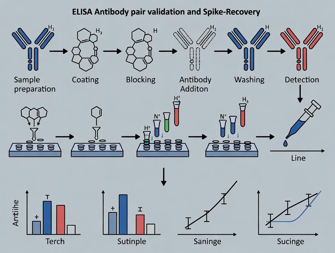
Visualizing Sandwich ELISA Architecture and Validation Workflow
Diagram 1: ELISA Architecture & Validation Workflow
Diagram 2: Spike-Recovery Experimental Logic
The Scientist's Toolkit: Key Research Reagent Solutions
Table 3: Essential Reagents for Sandwich ELISA Development & Validation
| Reagent / Material | Function / Purpose | Critical Consideration |
|---|---|---|
| Matched Antibody Pair | Provides the core specificity. Capture Ab immobilizes analyte; Detection Ab generates signal. | Must bind non-competing epitopes. Species/isotype differences reduce background. |
| Recombinant Purified Antigen | Serves as the standard for calibration curve generation and antibody titration. | Should be identical to the native target protein in epitope structure. |
| Blocking Protein (BSA, Casein) | Coats unused plastic surface to prevent non-specific binding of detection components. | Must be analyte- and antibody-free. Optimization required for each assay. |
| High-Affinity Streptavidin-Conjugate | Amplifies signal when using biotinylated detection antibodies (common 2-step detection). | High affinity reduces background; conjugate choice (HRP, AP) depends on substrate. |
| Chemiluminescent Substrate | Provides the detectable signal for HRP or Alkaline Phosphatase (AP) enzymes. | Offers wider dynamic range and higher sensitivity than colorimetric substrates. |
| Validated Biological Matrix | The sample diluent used for standards and samples (e.g., species-specific serum). | Must be characterized for minimal interference via spike-recovery experiments. |
| Microplates (High Binding) | Solid phase for antibody immobilization. | Consistent, high-binding capacity plates are essential for inter-assay precision. |
Key Characteristics of an Optimal Capture and Detection Antibody Pair
Within the broader thesis on ELISA antibody pair validation and spike-recovery experiments, the selection and validation of an optimal antibody pair is the foundational step determining assay sensitivity, specificity, and reliability. This document outlines the critical characteristics of such pairs and provides detailed protocols for their assessment.
Core Characteristics and Quantitative Comparison
Optimal antibody pairs must satisfy multiple, often competing, criteria. The following table synthesizes the key characteristics with target metrics derived from current literature and validation standards.
Table 1: Target Characteristics for an Optimal ELISA Antibody Pair
| Characteristic | Definition & Importance | Optimal Target / Benchmark |
|---|---|---|
| High Affinity | Equilibrium constant (KD) for antigen binding. Determines assay sensitivity and lower limit of detection (LLOD). | KD < 1 nM for both antibodies. |
| Specificity | Ability to bind exclusively to the target epitope without cross-reactivity to homologs, isoforms, or matrix proteins. | >99% specificity in a cross-reactivity panel. |
| Epitope Non-Overlap | Capture and detection antibodies must bind to distinct, non-competing epitopes on the target antigen. | Signal > 80% of maximum when both antibodies are co-incubated with antigen vs. individually. |
| Matched Sensitivity | Both antibodies should have similar affinity ranges to ensure efficient antigen "sandwiching." | Less than one log difference in monovalent KD values. |
| Low Lot-to-Lot Variability | Consistency in performance across different manufacturing lots. | Inter-lot CV < 15% for critical parameters (titer, sensitivity). |
| Matrix Tolerance | Maintains performance in complex biological samples (serum, plasma, cell lysate). | Spike recovery between 80-120% in relevant matrix. |
| Stability | Retains activity under standard storage and assay conditions. | >90% activity retained after 5 freeze-thaw cycles or long-term storage. |
Detailed Experimental Protocols
The following protocols are essential for validating these characteristics as part of a comprehensive thesis on assay development.
Protocol 1: Epitope Binning (Non-Overlap) Assay using ELISA
Objective: To confirm that the capture and detection antibodies bind to distinct, non-competing epitopes.
Materials:
- Purified target antigen
- Candidate capture antibody (Ab-C)
- Candidate detection antibody (Ab-D)
- HRP-conjugated secondary antibody (anti-species for Ab-D)
- ELISA plate, coating buffer, wash buffer, blocking buffer, TMB substrate, stop solution
Procedure:
- Coat plate with 100 µL/well of Capture Antibody (Ab-C) at 1-5 µg/mL in carbonate/bicarbonate buffer. Incubate overnight at 4°C.
- Block with 200 µL/well of protein-based blocking buffer (e.g., 3% BSA) for 1-2 hours at RT.
- Prepare Antigen-Antibody Mixtures: In separate tubes, pre-mix a fixed, saturating concentration of antigen with a serial dilution of unlabeled Detection Antibody (Ab-D). Include a control with antigen only.
- Transfer Mixtures: Add 100 µL of each pre-mix to the coated plate. Incubate for 2 hours at RT. (Directly adding Ab-D to the plate without pre-mixing is less conclusive).
- Wash plate 3x with wash buffer.
- Detect with appropriate HRP-conjugated secondary antibody against Ab-D. Incubate 1 hour at RT.
- Wash 3x.
- Develop with TMB substrate for 15-30 minutes. Stop with acid.
- Interpretation: If the detection signal remains high even at high concentrations of Ab-D in the pre-mix, it indicates non-competition (epitopes are distinct). A significant signal reduction indicates epitope overlap or steric hindrance.
Protocol 2: Spike-and-Recovery Experiment in Biological Matrix
Objective: To validate antibody pair performance in a complex sample matrix, a core component of the broader thesis.
Materials:
- Known concentration of purified antigen standard
- Antigen-negative biological matrix (e.g., normal human serum, plasma)
- Validated assay buffer (as calibrator diluent)
- Complete ELISA reagent set (validated pair, buffers)
Procedure:
- Prepare Spiked Samples:
- Neat Matrix Sample: Spike a high, mid, and low concentration of purified antigen into the natural matrix.
- Buffered Sample: Spike the same three concentrations into the assay buffer/calibrator diluent.
- Prepare a matching standard curve in assay buffer.
- Run the entire set of samples (spiked matrix, spiked buffer, standard curve) in the same ELISA plate in duplicate.
- Calculate the measured concentration for each spiked sample from the standard curve.
- Calculate Percent Recovery:
% Recovery = (Measured Concentration in Matrix / Measured Concentration in Buffer) x 100
- Validation Criterion: Acceptable recovery is typically 80-120%. Consistently low recovery suggests matrix interference; high recovery may indicate cross-reactivity.
Visualizing Antibody Pair Validation Workflow
Title: Antibody Pair Validation Workflow for ELISA
The Scientist's Toolkit: Essential Research Reagent Solutions
Table 2: Key Reagents for Antibody Pair Validation
| Reagent / Solution | Function in Validation | Critical Consideration |
|---|---|---|
| Biacore or Octet Systems | Label-free kinetic analysis (KD, kon, koff) for affinity determination. | Requires purified antigen and antibodies. High-quality data is gold standard for affinity. |
| MSD / Electrochemiluminescence Plates | High-sensitivity platform for preliminary pairing screening with broad dynamic range. | Useful for testing multiple candidates in small sample volumes. |
| Cross-Reactivity Protein Panel | Recombinant proteins from the same family or homologs to test specificity. | Must include closest phylogenetic relatives and common matrix proteins. |
| Stable, Purified Antigen | The critical standard for all quantitative experiments (spike recovery, calibration). | Must be in native conformation, highly pure, and accurately quantified. |
| Matrix-Blanked Diluent | Specialized assay buffer designed to minimize matrix effects (e.g., contains blockers, heterophilic blockers). | Essential for achieving 80-120% spike recovery in complex samples. |
| Precision and Recovery Controls | QC samples (low, mid, high concentration) in relevant matrix. | Used for inter-assay precision monitoring and long-term validation stability. |
| HRP or ALP Conjugation Kits | For in-house labeling of detection antibodies, allowing for pair customization. | Consistency in degree of labeling (DOL) is key to reproducible sensitivity. |
Understanding Epitope Mapping and Avoiding Steric Hindrance in Pair Selection
Within the broader thesis on ELISA antibody pair validation and spike-recovery experiments, epitope mapping and steric hindrance avoidance are critical for developing robust, quantitative sandwich immunoassays. The selection of matched antibody pairs—where a capture antibody and a detection antibody bind non-competitively to the same target antigen—directly dictates assay sensitivity, specificity, and dynamic range. This Application Note details protocols and considerations for successful pair selection.
Key Principles: Epitope Mapping and Steric Hindrance
- Epitope Mapping: The process of identifying the specific binding site (epitope) of an antibody on the target antigen. For sandwich ELISAs, antibodies must bind to distinct, non-overlapping epitopes.
- Steric Hindrance: The physical blockage of one antibody's binding site due to the proximity of another bound antibody, even if epitopes are not identical. This prevents the formation of the sandwich complex.
Experimental Protocols for Pair Validation
Protocol 3.1: Epitope Binning via Sequential ELISA
Objective: To determine if two monoclonal antibodies bind to overlapping or non-overlapping epitopes. Materials: 96-well ELISA plate, antigen, candidate antibody pairs, blocking buffer, HRP-conjugated secondary antibody, TMB substrate, stop solution, plate reader. Procedure:
- Coat plate with antigen (or capture antibody if antigen is scarce). Incubate overnight at 4°C.
- Block plate with protein-based blocking buffer (e.g., 3% BSA) for 1-2 hours at room temperature (RT).
- Add saturating concentration of first candidate antibody (Ab-A). Incubate 1-2 hours at RT.
- Without washing, add HRP-conjugated second candidate antibody (Ab-B) at a defined concentration. Incubate 1 hour at RT.
- Wash plate thoroughly.
- Develop with TMB substrate for 15-30 minutes. Stop reaction and read absorbance at 450nm.
- Interpretation: A high signal indicates Ab-B can bind simultaneously with Ab-A (non-overlapping epitopes, low steric hindrance). A low signal suggests epitope overlap or steric hindrance.
- Reverse the order (Ab-B first, then HRP-conjugated Ab-A) to confirm.
Protocol 3.2: Checkerboard Titration for Pair Optimization
Objective: To determine the optimal concentration combination for a candidate matched pair identified as non-overlapping. Procedure:
- Prepare a dilution series of the capture antibody (e.g., 10, 5, 2.5, 1.25 µg/mL) in coating buffer.
- Coat rows of a plate with different capture antibody concentrations. Incubate and block as standard.
- Add a fixed, high concentration of antigen to all wells.
- Prepare a dilution series of the detection antibody (e.g., 5, 2.5, 1.25, 0.625 µg/mL).
- Add different detection antibody concentrations to columns of the plate.
- Proceed with standard detection steps (secondary antibody if needed, substrate).
- Analyze the signal-to-background ratio for each combination to identify the concentration pair that yields the highest specific signal with lowest background.
Data Presentation: Quantitative Pair Validation
Table 1: Sequential ELISA Epitope Binning Results
| Antibody Pair (Capture → Detection) | OD 450nm | Interpretation |
|---|---|---|
| mAb-A → mAb-B (conj.) | 2.85 | Non-overlapping |
| mAb-B → mAb-A (conj.) | 2.90 | Non-overlapping |
| mAb-A → mAb-C (conj.) | 0.15 | Overlapping/Hindered |
| mAb-C → mAb-A (conj.) | 0.22 | Overlapping/Hindered |
Table 2: Checkerboard Titration for Optimal Concentrations
| Capture [µg/mL] | Detection Antibody Concentration [µg/mL] | |||
|---|---|---|---|---|
| 5.0 | 2.5 | 1.25 | 0.625 | |
| 10.0 | 3.2* | 3.0 | 2.7 | 2.1 |
| 5.0 | 3.0 | 2.9 | 2.6 | 1.9 |
| 2.5 | 2.6 | 2.5 | 2.3 | 1.5 |
| 1.25 | 1.8 | 1.7 | 1.5 | 0.9 |
*OD 450nm values. Highlighted cell indicates optimal concentration pair (10 µg/mL capture, 5 µg/mL detection) offering highest signal before plateau.
The Scientist's Toolkit: Essential Reagent Solutions
Table 3: Key Research Reagents for Epitope Mapping & Pair Validation
| Reagent / Material | Function in Experiment |
|---|---|
| Monoclonal Antibody Pairs | Provide specificity to distinct epitopes; essential for sandwich assay development. |
| Recombinant Antigen | Pure, well-characterized antigen for controlled coating and binning experiments. |
| HRP-Conjugated Antibodies | Enable direct detection in sequential ELISAs or via secondary amplification. |
| Chromogenic TMB Substrate | Generates measurable colorimetric signal upon enzymatic reaction with HRP. |
| Magnetic Bead-Based Binning Kits | (Alternative) Streamline epitope binning via competitive binding assays on bead surfaces. |
| Biacore/SPR Chips | (Advanced) Label-free real-time kinetics analysis for detailed epitope mapping and affinity measurements. |
Visualization of Workflows
Diagram 1: Sequential ELISA Binning Workflow
Diagram 2: Steric Hindrance vs. Valid Pair Binding
The Central Role of Spike-Recovery Experiments in Assessing Assay Accuracy and Matrix Effects
Within the rigorous framework of ELISA antibody pair validation, the spike-recovery experiment stands as a cornerstone analytical procedure. This protocol is critical for a broader thesis investigating the reliability of quantitative immunoassays in biotherapeutic and biomarker development. It directly interrogates two fundamental parameters: accuracy (the closeness of measured value to the true value) and the presence of matrix effects (interference from sample components like proteins, lipids, or salts that can alter the assay signal). Accurate recovery of a known quantity of analyte spiked into a relevant biological matrix validates the assay's performance in its intended context and confirms the suitability of the matched antibody pair.
Application Notes: Principles and Interpretation
Core Objectives
- Quantify Accuracy: Determine if the assay correctly measures the analyte concentration across its dynamic range within the specific sample type (e.g., serum, plasma, cell lysate).
- Identify Matrix Effects: Diagnose signal suppression or enhancement caused by the sample matrix, which can lead to under- or over-reporting of analyte concentration.
- Validate Dilution Linearity: Establish that samples can be reliably diluted in assay buffer or a designated diluent to bring readings into the assay's quantifiable range.
Key Performance Metrics
Acceptance criteria for spike-recovery are typically derived from industry white papers and guidelines (e.g., ICH, CLSI). A common benchmark for ligand-binding assays like ELISA is:
- Mean Recovery: 80–120% of the expected value.
- Precision (CV): ≤20% across replicates.
Data falling outside these ranges indicate significant matrix interference or assay incompatibility, necessitating protocol optimization such as sample pre-treatment, alternative diluents, or antibody pair re-evaluation.
Table 1: Representative Spike-Recovery Data for a Cytokine ELISA in Human Serum
| Sample Matrix | Endogenous [Analyte] (pg/mL) | Spike Amount Added (pg/mL) | Expected [Total] (pg/mL) | Measured [Total] (Mean ± SD, pg/mL) | % Recovery | CV (%) |
|---|---|---|---|---|---|---|
| Assay Buffer (Neat) | 0.0 | 50.0 | 50.0 | 49.8 ± 2.1 | 99.6 | 4.2 |
| Normal Human Serum (1:2 Dil) | 15.2 | 50.0 | 65.2 | 58.1 ± 4.5 | 89.1 | 7.7 |
| Normal Human Serum (1:4 Dil) | 7.6* | 50.0 | 57.6 | 53.9 ± 3.1 | 93.6 | 5.8 |
| Diseased Patient Serum (1:10 Dil) | 125.0 | 100.0 | 225.0 | 192.3 ± 18.7 | 85.5 | 9.7 |
*Calculated based on dilution factor.
Table 2: Recovery Acceptance Criteria by Sample Type
| Sample Type / Context | Recommended Recovery Range | Typical Dilution Factor Range | Primary Concern |
|---|---|---|---|
| Tier 1: Validated Reference Standard in Buffer | 95–105% | N/A | Assay intrinsic accuracy |
| Tier 2: Normal Individual Matrices | 80–120% | 2–10x | Moderate matrix components |
| Tier 3: Diseased/Stressed Matrices | 70–130%* | 10–100x | High analyte levels, heterophilic antibodies, severe interference |
*May require extensive sample pre-treatment or alternative assay format.
Detailed Experimental Protocols
Protocol A: Basic Spike-Recovery and Parallelism Assessment
Objective: To assess accuracy and matrix effects across the assay range.
Materials: (See Scientist's Toolkit) Procedure:
- Prepare Spiked Samples:
- Aliquot a volume of the biological matrix (e.g., serum pool) into three tubes.
- Tube 1 (Baseline): Add an equal volume of sample diluent (zero spike).
- Tube 2 (Mid Spike): Add an equal volume of sample diluent containing the analyte at a concentration 2x the intended mid-level spike concentration.
- Tube 3 (High Spike): Add an equal volume of sample diluent containing the analyte at a concentration 2x the intended high-level spike concentration.
- Mix thoroughly. The final dilution of the matrix is now 1:2, with the target spike levels achieved.
Prepare Calibrators and QCs: Dilute the reference standard in assay buffer per the standard ELISA protocol.
Assay Execution: Run the spiked samples, calibrators, and QC samples in the same ELISA plate according to the validated protocol (coat, block, sample incubation, detection antibody, enzyme conjugate, substrate, stop).
Data Analysis:
- Generate a standard curve from the calibrators (typically 4- or 5-parameter logistic fit).
- Interpolate the measured concentration of the spiked samples from the curve.
- Calculate % Recovery:
% Recovery = (Measured [Spiked] – Measured [Baseline]) / Theoretical Spike Amount * 100. - Assess Parallelism: Serial dilute a high-concentration native matrix sample (or a high-spike sample) in assay diluent. The calculated concentrations, when adjusted for dilution, should be constant (± acceptable CV). Non-parallelism indicates matrix interference.
Protocol B: Dilutional Linearity to Overcome Matrix Effects
Objective: To determine the optimal dilution factor that minimizes interference.
Procedure:
- Prepare a series of dilutions (e.g., 1:2, 1:4, 1:8, 1:16, 1:32) of the spiked matrix sample in the chosen assay diluent.
- Assay all dilutions alongside the standard curve.
- Plot the observed concentration (from the curve) against the dilution factor. The plot should be linear and pass through the origin for an ideal, interference-free system.
- Identify the dilution range where recovery falls within the 80–120% acceptance criteria. This defines the validated dilution range for the assay for that specific matrix.
Visualizations
The Scientist's Toolkit: Research Reagent Solutions
| Item | Function in Spike-Recovery Experiments | Key Considerations |
|---|---|---|
| Matched Antibody Pair | Capture and detection antibodies specific to the target analyte. Forms the core of the ELISA. | Affinity, specificity, and lot-to-lot consistency are paramount. Must be validated as a pair. |
| Reference Standard (Pure Analyte) | Highly purified protein of known concentration and activity. Used for spiking and standard curve generation. | Must be traceable to a primary standard. Stability and reconstitution accuracy are critical. |
| Relevant Biological Matrix | The actual sample type the assay is designed for (e.g., human serum, mouse plasma, cell culture supernatant). | Pooled samples from multiple donors are used to assess "normal" matrix effects. |
| Assay Buffer / Sample Diluent | The buffer used to dilute samples, standards, and reagents. Often contains proteins (BSA) and detergents. | Optimized to minimize non-specific binding and stabilize the analyte. Critical for overcoming matrix interference. |
| Interference-Blocking Reagents | Additives like heterophilic blocking reagent, protease inhibitors, or specific binding protein competitors (e.g., soluble receptor). | Added to sample diluent to neutralize common interferants like heterophilic antibodies or binding proteins. |
| Pre-coated ELISA Plates | Microplates with capture antibody already immobilized. | Ensure consistency and save time. Check binding capacity and stability. |
| Precision Pipettes & Liquid Handler | For accurate and reproducible transfer of samples, spikes, and reagents. | Essential for generating reliable serial dilutions and ensuring accurate spike volumes. |
| Plate Reader with Analysis Software | Measures absorbance (or other signal) and facilitates curve fitting and interpolation. | Software should support 4PL/5PL regression for accurate quantification across a wide range. |
Within the rigorous framework of ELISA antibody pair validation and spike-recovery experiments for biotherapeutics development, establishing robust analytical methods is paramount. The reliability of pharmacokinetic (PK), immunogenicity, and biomarker data hinges on the thorough validation of the assay itself. This document defines and outlines experimental protocols for four foundational validation parameters: Specificity, Sensitivity, Dynamic Range, and Parallelism. These parameters are critical for ensuring that an ELISA measures the intended analyte accurately, precisely, and reproducibly across the relevant biological matrix and concentration spectrum, thereby supporting regulatory filings and clinical decision-making.
Key Parameter Definitions and Experimental Protocols
Specificity
Definition: The ability of the assay to exclusively measure the target analyte without interference from structurally similar molecules, cross-reactive matrix components, or therapeutic agents (e.g., concomitant drugs). Thesis Relevance: Validates the antibody pair's selectivity for the target protein in the presence of serum/plasma proteins, soluble receptors, homologous proteins, or anti-drug antibodies (ADAs).
Protocol: Interference Testing
- Sample Preparation: Prepare pools of the relevant biological matrix (e.g., normal human serum). Spike with:
- The target analyte at a medium concentration (within the quantitative range).
- Potential interfering substances at physiologically or pathologically relevant high concentrations (e.g., soluble receptors, homologous proteins, rheumatoid factor, biotin, lipids).
- A combination of the target analyte and each interfering substance. Include control samples: analyte-only spike and matrix-only.
- Assay: Run all samples in the ELISA according to the established protocol.
- Data Analysis: Calculate % recovery for the analyte spiked in the presence of the interferent.
- Recovery (%) = (Measured conc. of analyte with interferent / Measured conc. of analyte alone) x 100. Acceptance criterion is typically 80-120% recovery, demonstrating a lack of interference.
Sensitivity
Definition: The lowest concentration of the analyte that can be reliably distinguished from zero. It is practically defined as the Lower Limit of Detection (LLOD) and the Lower Limit of Quantification (LLOQ). Thesis Relevance: Determines the assay's capability to detect low analyte levels, crucial for PK tail characterization and low-titer ADA assessments.
Protocol: LLOQ Determination
- Sample Preparation: Prepare at least 10 independent replicates of the biological matrix spiked with the analyte at the putative LLOQ (a very low concentration expected to be near the assay's limit). Also prepare replicates of the blank matrix (zero analyte).
- Assay: Analyze all replicates in a single run.
- Data Analysis:
- LLOD: Often calculated as the mean signal of the blank + 3 (Standard Deviations).
- LLOQ: The lowest concentration where: a) %CV of replicates is ≤ 20% (or 25% for ligand-binding assays). b) Mean recovery is within 80-120%. c) The signal is distinguishable from the blank (e.g., mean signal > mean blank signal + 10*SD of blank).
Dynamic Range
Definition: The span of analyte concentrations between the LLOQ and the Upper Limit of Quantification (ULOQ) that can be measured with acceptable accuracy and precision. It is defined by the standard curve. Thesis Relevance: Ensures the assay can quantify analyte concentrations across the entire expected range from pre-dose to peak levels in PK studies without sample dilution.
Protocol: Standard Curve and ULOQ Validation
- Sample Preparation: Prepare a standard curve using a serial dilution of the analyte in assay buffer and in the biological matrix. The highest point should exceed the expected maximum concentration.
- Assay: Run the standard curve in replicate (e.g., n=3) across multiple runs/days.
- Data Analysis:
- Fit the calibration curve using an appropriate model (e.g., 4- or 5-parameter logistic).
- ULOQ: The highest concentration where: a) %CV of back-calculated concentrations is ≤ 20% (or 25%). b) Mean recovery is within 80-120%.
- The Dynamic Range is reported as LLOQ to ULOQ (e.g., 10 ng/mL – 1000 ng/mL).
Parallelism
Definition: The demonstration that the diluted sample behaves immunochemically identically to the standard curve. It assesses the absence of matrix effects that distort measurement at different dilutions. Thesis Relevance: Validates that sample dilution, a routine practice for bringing high-concentration samples into range, yields accurate results, confirming the standard curve is appropriate for real samples.
Protocol: Parallelism Dilutional Linearity
- Sample Preparation: Select at least 3 individual or pooled matrix samples with endogenous or spiked high analyte levels. Perform a serial dilution (e.g., 1:2, 1:4, 1:8, etc.) using the appropriate blank matrix to bring concentrations within the assay range.
- Assay: Analyze all dilutions of each sample alongside the standard curve.
- Data Analysis: Plot measured concentration (corrected for dilution factor) vs. dilution factor. Assess linearity and calculate % recovery at each dilution level relative to the expected concentration.
- Acceptance: %CV of the back-calculated concentrations across dilutions should be ≤ 20-30%, and the slope of the regression line should be near zero.
Data Presentation Tables
Table 1: Specificity/Interference Testing Results
| Interferent Tested | Conc. of Interferent | % Recovery of Target Analyte | Conclusion (Pass/Fail) |
|---|---|---|---|
| Soluble Receptor X | 100 ng/mL | 102% | Pass |
| Homologous Protein Y | 50 µg/mL | 135% | Fail (Cross-reactivity) |
| Rheumatoid Factor | 500 IU/mL | 95% | Pass |
| Lipemic Serum (Intralipid) | 3% v/v | 88% | Pass |
| Biotin | 100 ng/mL | 110% | Pass |
Table 2: Sensitivity and Dynamic Range Summary
| Parameter | Value | Acceptance Criteria | Result |
|---|---|---|---|
| LLOD | 1.5 ng/mL | Signal > Blank Mean + 3SD | Established |
| LLOQ | 5.0 ng/mL | CV ≤20%, Recovery 80-120% | Established |
| ULOQ | 800 ng/mL | CV ≤20%, Recovery 80-120% | Established |
| Dynamic Range | 5 - 800 ng/mL | LLOQ to ULOQ | >2 logs |
Table 3: Parallelism Assessment of a High-Titer Sample
| Sample Dilution | Measured Conc. (ng/mL) | Dilution-Corrected Conc. (ng/mL) | % Recovery vs. Predicted |
|---|---|---|---|
| 1:10 | 78.5 | 785 | 98.1% |
| 1:20 | 38.9 | 778 | 97.3% |
| 1:40 | 19.8 | 792 | 99.0% |
| 1:80 | 9.9 | 792 | 99.0% |
| Mean ± %CV | 786.8 ± 1.0% | 98.4 ± 0.9% |
Detailed Experimental Protocol: Parallelism Testing for an Anti-TNFα mAb ELISA
Title: Protocol for Assessing Parallelism in a Serum-Based Anti-TNFα Therapeutic ELISA.
Objective: To validate that human serum samples containing a therapeutic anti-TNFα monoclonal antibody can be accurately quantified across multiple dilutions.
Materials: (See The Scientist's Toolkit below).
Procedure:
- Preparation of High-Concentration QC Samples: Pool sera from relevant subjects or spike the anti-TNFα mAb into normal human serum to create three High QC pools (HQC1, HQC2, HQC3) with concentrations near the expected ULOQ.
- Dilution Series: For each HQC pool, perform a 4-fold serial dilution in blank (analyte-free) normal human serum. Create at least 4 dilutions per pool (e.g., 1:4, 1:16, 1:64, 1:256). Ensure the final dilutions fall within the validated quantitative range (5-800 ng/mL).
- Plate Analysis:
- Run a standard curve in duplicate (from 800 ng/mL to 5 ng/mL, prepared in blank serum).
- Run all dilutions of the three HQC pools in duplicate.
- Include system suitability controls (LLOQ, Low, Mid, High QCs).
- Calculations:
- Generate the standard curve using a 5-PL curve fit.
- Calculate the concentration of each diluted sample.
- Multiply each result by its dilution factor to obtain the original, undiluted concentration.
- Acceptance Criteria: The calculated %CV of the undiluted concentrations across all valid dilutions for each pool must be ≤ 25%. Individual dilution recoveries should be within 75-125%.
Visualizations
Diagram Title: ELISA Validation Parameter Workflow and Decision Logic.
Diagram Title: Relationship Between Dynamic Range, Standard Curve, and Parallelism.
The Scientist's Toolkit: Key Reagent Solutions
| Item | Function in Validation Experiments |
|---|---|
| Matched Antibody Pair | Capture and detection antibodies specific to the target analyte; the core of assay specificity. |
| Recombinant Target Protein | Used as the standard for calibration curves and for spiking into matrices for recovery studies. |
| Control Matrix | Analyte-free biological fluid (e.g., charcoal-stripped serum) for preparing standards and diluents. |
| Interferent Stocks | Purified proteins (e.g., soluble receptors, homologs), lipids, biotin, or ADA positive controls for specificity tests. |
| Blocking Buffer | Protein-based solution (e.g., BSA, casein) to prevent nonspecific binding to the plate. |
| HRP-Conjugated Detection Ab | Enzyme-linked antibody for signal generation in a sandwich ELISA format. |
| Chemiluminescent Substrate | Provides sensitive, wide dynamic range signal for detection and LLOQ determination. |
| Microplate Washer & Reader | Automation for consistent washing steps and accurate optical or luminescent signal measurement. |
| Statistical Software (e.g., SoftMax Pro, PLA) | For curve fitting, data analysis, and calculation of validation parameters (LLOQ, %CV, %Recovery). |
Step-by-Step Protocols: Executing Antibody Pair Titration and Spike-Recovery Experiments for Precision Data
Within the broader thesis on ELISA antibody pair validation and spike-recovery experiments, the precise optimization of capture and detection antibody concentrations is a critical foundational step. A systematic checkerboard titration is the definitive method to identify the optimal concentration pair that yields the highest signal-to-noise ratio, ensuring maximum assay sensitivity and specificity for subsequent validation and recovery studies. This protocol details the application of this method for sandwich ELISA development.
The Scientist's Toolkit: Essential Research Reagent Solutions
| Item | Function in Checkerboard Titration |
|---|---|
| High-Purity Capture Antibody | Immobilized on the plate to specifically bind the target analyte. Concentration is varied along one axis of the checkerboard. |
| High-Purity Detection Antibody | Binds to a different epitope on the captured analyte. Conjugated to an enzyme (e.g., HRP). Concentration is varied along the other axis. |
| Recombinant Target Antigen | The protein of interest used for titration. A known, high-purity standard is essential for accurate optimization. |
| Blocking Buffer (e.g., 5% BSA) | Prevents non-specific binding of antibodies to the plate, reducing background signal. |
| HRP Substrate (e.g., TMB) | Chromogenic substrate for horseradish peroxidase (HRP). Produces a measurable color change proportional to detection antibody binding. |
| Stop Solution (e.g., 1M H₂SO₄) | Terminates the enzymatic reaction, stabilizing the final absorbance for reading. |
| Microplate Washer | Ensures consistent and thorough removal of unbound reagents between steps, critical for low background. |
| Plate Reader (450 nm) | Precisely measures the absorbance of the developed chromogenic substrate. |
Detailed Experimental Protocol
Materials Preparation
- Coating Buffer: 0.05 M Carbonate-Bicarbonate, pH 9.6.
- Wash Buffer: PBS containing 0.05% Tween 20 (PBST).
- Diluent Buffer: PBS containing 1% BSA.
- Antigen Solution: Prepare the target antigen at a concentration near the expected mid-point of the assay range (e.g., 100-500 pg/mL) in diluent buffer.
Checkerboard Titration Procedure
- Plate Coating (Capture Antibody Titration):
- Prepare a dilution series of the capture antibody in coating buffer (e.g., 10, 5, 2.5, 1.25, 0.625 µg/mL).
- Dispense 100 µL of each concentration into the columns of a 96-well microplate in triplicate, following a layout where columns represent different capture antibody concentrations.
- Seal and incubate overnight at 4°C.
- Washing & Blocking:
- Aspirate and wash plates 3x with wash buffer.
- Add 300 µL of blocking buffer per well. Incubate for 1-2 hours at room temperature (RT).
- Wash plate 3x.
- Antigen Addition:
- Add 100 µL of the prepared antigen solution to all wells. Include wells with diluent only as background controls.
- Incubate for 2 hours at RT.
- Wash plate 3-5x.
- Detection Antibody Titration:
- Prepare a dilution series of the detection antibody in diluent buffer (e.g., 2, 1, 0.5, 0.25, 0.125 µg/mL).
- Dispense 100 µL of each concentration into the rows of the plate, creating a matrix (checkerboard) where each well contains a unique pair of capture and detection antibody concentrations.
- Incubate for 1-2 hours at RT.
- Wash plate 5x.
- Signal Detection:
- Add 100 µL of HRP substrate (e.g., TMB) per well. Incubate in the dark for 10-20 minutes.
- Stop the reaction with 50-100 µL of stop solution.
- Read the absorbance immediately at 450 nm (with a reference wavelength of 570-650 nm).
Data Analysis
- Calculate the mean absorbance for each condition (antibody pair).
- Subtract the mean background signal (wells with no antigen) from all values.
- Plot the signal (corrected absorbance) for each detection antibody concentration across the different capture antibody concentrations.
Table 1: Example Checkerboard Titration Results (Corrected Absorbance at 450 nm) Target Antigen Concentration: 250 pg/mL
| Detection [µg/mL] → Capture [µg/mL] ↓ | 2.0 | 1.0 | 0.5 | 0.25 | 0.125 |
|---|---|---|---|---|---|
| 10.0 | 3.210 | 2.980 | 2.401 | 1.555 | 0.801 |
| 5.0 | 3.105 | 3.150 | 2.650 | 1.720 | 0.902 |
| 2.5 | 2.850 | 2.950 | 2.800 | 1.950 | 1.050 |
| 1.25 | 2.301 | 2.500 | 2.601 | 2.100 | 1.201 |
| 0.625 | 1.502 | 1.803 | 2.000 | 1.850 | 1.302 |
| 0 (Background) | 0.101 | 0.098 | 0.105 | 0.099 | 0.102 |
Optimal Condition Selection: The optimal pair is typically chosen from the plateau region offering the highest signal with the lowest background. In this example, Capture: 2.5 µg/mL & Detection: 0.5 µg/mL provides a high signal (2.800) while conserving valuable antibody reagents compared to higher concentration pairs.
Visualized Workflows and Pathways
Checkerboard Titration Workflow
Optimal Pair Selection Logic
Within the rigorous validation of ELISA antibody pairs for quantifying biomarkers in complex biological matrices, the spike-recovery experiment is a cornerstone assay. It directly assesses accuracy by determining the ability of the assay to measure an analyte of interest (the "spike") when added to a sample. This protocol details the design and execution of these experiments, focusing on spiking strategies and the implementation of a control matrix. The findings are integral to a broader thesis establishing standardized, reliable frameworks for immunoassay validation in drug development, ensuring that pharmacokinetic, pharmacodynamic, and safety biomarker data are accurate and reproducible.
Key Principles and Definitions
- Spike: A known, purified quantity of the target analyte (antigen) added to a sample matrix.
- Endogenous Concentration: The analyte concentration naturally present in the sample matrix before spiking.
- Matrix: The biological fluid (e.g., serum, plasma, tissue homogenate, cell culture supernatant) containing the sample.
- Spike Recovery: The percentage of the measured (observed) spike concentration relative to the expected (theoretical) spike concentration.
- Formula: Recovery (%) = [(Observed Concentration in Spiked Sample) – (Observed Concentration in Unspiked Sample)] / (Theoretical Spike Concentration) × 100.
- Control Matrix: A matrix that is confirmed or presumed to have negligible endogenous levels of the target analyte, used to establish the baseline for recovery calculations (e.g., analyte-depleted serum, buffer, or a different species' matrix).
Experimental Design: Spiking Strategies and Control Matrices
The core design involves preparing a series of samples with known spike levels and comparing the measured values to the expected values.
3.1. Selection of Spiking Concentrations: Spikes should cover the assay's dynamic range, with emphasis on the low, mid, and high regions of the standard curve. A minimum of three spike levels (in replicates, typically n=3-5) is required for a robust assessment.
3.2. The Parallelism vs. Spiked-Recovery Strategy: Two primary approaches exist, as summarized in Table 1.
Table 1: Comparison of Spiking Strategies
| Strategy | Matrix Used | Purpose | Calculation | Ideal Recovery Range |
|---|---|---|---|---|
| Spike Recovery in Control Matrix | Analyte-free or surrogate matrix (e.g., buffer, charcoal-stripped serum). | Assesses inherent assay accuracy without interference from endogenous matrix components. | (Measured Spike in Control Matrix) / (Theoretical Spike) x 100. | 80–120% (or 75–125% at LLOQ/ULOQ). |
| Spike Recovery in Study Matrix | The actual biological sample of interest (e.g., patient serum). | Assesses overall accuracy in the presence of endogenous analyte and all matrix effects. | [(Spiked Sample) – (Unspiked Sample)] / (Theoretical Spike) x 100. | 80–120% (or 75–125% at LLOQ/ULOQ). |
| Parallelism (Dilutional Linearity) | Study matrix with high endogenous levels. | Validates that the sample dilution behavior parallels the standard curve, confirming absence of matrix interference. | Observed concentration after dilution aligns with expected dilution factor. | Consistency across dilutions (e.g., %CV <20-25%). |
3.3. The Control Matrix Experiment Workflow: A systematic workflow is required to differentiate matrix effects from assay performance.
(Diagram Title: Control Matrix vs Study Matrix Experimental Flow)
Detailed Experimental Protocol
4.1. Materials and Reagents (The Scientist's Toolkit) Table 2: Essential Research Reagent Solutions
| Item | Function / Description |
|---|---|
| Purified Target Antigen (Lyophilized Standard) | The "spike" material. Must be highly purified and of known concentration. Reconstituted in a compatible buffer. |
| Candidate ELISA Kit/Antibody Pair | The immunoassay components under validation, including capture antibody, detection antibody, and conjugate. |
| Study Matrix (Biological Sample) | The test matrix containing (potentially) endogenous analyte. Should be representative (e.g., pooled from multiple donors). |
| Control Matrix | Matrix with minimal endogenous analyte. Can be commercial analyte-depleted serum, assay buffer, or a heterologous species matrix. |
| Assay Diluent / Sample Buffer | The buffer used to dilute samples and standards. Optimized to minimize nonspecific binding and matrix interference. |
| Calibration Standard Series | A dilution series of the purified antigen in assay diluent, used to generate the standard curve. |
| Microplate Washer & Reader | Equipment for automated washing and precise absorbance measurement. |
4.2. Step-by-Step Procedure
A. Preparation:
- Reconstitution & Dilution: Reconstitute the purified antigen standard per manufacturer instructions. Prepare a high-concentration "spiking stock" solution in an appropriate buffer.
- Spiking Intermediate Solutions: Serially dilute the spiking stock to create at least three intermediate working solutions (High, Mid, Low) that, when added to the matrix, will yield final concentrations within the desired range (e.g., near the LLOQ, mid-point, and 80% of the ULOQ of the standard curve).
- Matrix Aliquoting: Aliquot the required volume of Study Matrix and Control Matrix into separate tubes. Include extra aliquots for unspiked controls.
B. Spiking:
- Low-Volume Spiking: Add a small, precise volume (e.g., ≤10% of total sample volume) of each spiking intermediate solution to the matrix aliquots. For the Study Matrix, spike into separate aliquots.
- Unspiked Controls: Add an equivalent volume of spiking buffer (without analyte) to separate aliquots of both Study and Control Matrices.
- Vortex & Incubate: Mix thoroughly and incubate for 15-30 minutes at room temperature to allow equilibration of the spike with the matrix.
- Final Dilution (if needed): Perform any required pre-assay dilutions of the spiked samples using the assay diluent.
C. Assay Execution:
- Run the ELISA according to the optimized protocol.
- Include the full Calibration Standard Series in duplicate on the same plate.
- Run all spiked samples, unspiked controls, and matrix blanks (assay diluent only) in appropriate replicates (minimum n=3).
- Plate Layout: Utilize a randomized or balanced plate layout to minimize positional effects.
D. Data Analysis:
- Generate a 4- or 5-parameter logistic (4PL/5PL) standard curve from the calibration standards.
- Interpolate the observed concentration for all samples from the curve.
- Calculate % Recovery for each spike level using the formulas in Section 2.
- Compile data into summary tables.
Table 3: Example Spike-Recovery Data Output
| Matrix Type | Spike Level | Theoretical [Spike] | Mean Observed [Total] | Mean Observed [Unspiked] | Mean Observed [Spike] | % Recovery | %CV (n=3) |
|---|---|---|---|---|---|---|---|
| Control Matrix | Low | 5.0 pg/mL | 4.8 pg/mL | 4.8 pg/mL | 96.0% | 6.2% | |
| (Buffer) | Mid | 50 pg/mL | 52.1 pg/mL | 52.1 pg/mL | 104.2% | 4.5% | |
| High | 400 pg/mL | 388.0 pg/mL | 388.0 pg/mL | 97.0% | 3.8% | ||
| Study Matrix | Low | 5.0 pg/mL | 8.2 pg/mL | 3.5 pg/mL | 4.7 pg/mL | 94.0% | 8.1% |
| (Human Serum) | Mid | 50 pg/mL | 60.1 pg/mL | 3.5 pg/mL | 56.6 pg/mL | 113.2% | 5.7% |
| High | 400 pg/mL | 410.3 pg/mL | 3.5 pg/mL | 406.8 pg/mL | 101.7% | 4.9% |
Interpretation and Troubleshooting
- Acceptance Criteria: Recovery of 80–120% (with wider bounds at extremes) and a precision (%CV) of <20% (or <25% at LLOQ) are commonly targeted.
- Low Recovery in Control Matrix: Suggests fundamental assay issues: antibody affinity/avidity problems, spike instability, or interference from the control matrix itself.
- Acceptable Recovery in Control but Poor Recovery in Study Matrix: Indicates significant matrix interference specific to the study sample. Requires mitigation via sample dilution, alternative sample pre-treatment, or antibody pair re-evaluation.
- High Recovery (>120%): May indicate cross-reactivity, hook effect at high concentrations, or calibration standard inaccuracy.
- The Role of Parallelism: The relationship between spiking strategies is visualized in the decision logic below.
(Diagram Title: Spike-Recovery and Parallelism Decision Logic)
Conclusion: A meticulously designed spike-recovery experiment, utilizing appropriate control matrices and spiking strategies, is non-negotiable for validating ELISA antibody pairs. This protocol provides a structured framework to generate defensible data on assay accuracy, directly informing the reliability of downstream research and drug development decisions.
Application Notes & Protocols
Within the broader thesis on ELISA antibody pair validation and spike-recovery experiments, establishing and interpreting percentage recovery is a critical performance metric. It quantifies the accuracy of an analytical method by measuring how much of a known, added amount of analyte (the "spike") is recovered from a test sample. Acceptable recovery limits (typically 80-120%) are essential for validating immunoassays in drug development, ensuring reliable quantification of biomarkers, therapeutic proteins, or contaminants in complex biological matrices.
Core Formula & Interpretation
Percentage Recovery Calculation:
% Recovery = (Measured Concentration of Spiked Sample − Measured Concentration of Unspiked Sample) / Theoretical Spike Concentration × 100
Interpretation of Limits (80-120%):
- Recovery < 80%: Suggests potential matrix interference (e.g., binding proteins, proteases, pH differences), analyte loss (adsorption, degradation), or antibody cross-reactivity issues.
- Recovery within 80-120%: Generally indicates acceptable method accuracy for the tested matrix and concentration. The specific target (e.g., 85-115%) should be defined a priori based on assay requirements.
- Recovery > 120%: May indicate signal enhancement from the matrix, calibration standard inaccuracy, or hook effect at high concentrations.
Table 1: Hypothetical Spike-Recovery Data for an IL-6 ELISA in Rat Serum
| Sample Matrix | Endogenous [IL-6] (pg/mL) | Spike Added (pg/mL) | Expected [IL-6] (pg/mL) | Measured [IL-6] (pg/mL) | % Recovery | Acceptable (80-120%)? |
|---|---|---|---|---|---|---|
| Rat Serum Pool 1 | 25.2 | 50.0 | 75.2 | 71.1 | 91.8% | Yes |
| Rat Serum Pool 1 | 25.2 | 200.0 | 225.2 | 240.5 | 107.7% | Yes |
| Rat Serum Pool 2 | 10.5 | 50.0 | 60.5 | 44.7 | 68.4% | No |
| Assay Buffer (Control) | 0.0 | 50.0 | 50.0 | 49.0 | 98.0% | Yes |
Table 2: Statistical Summary of Recovery Across Validation Runs
| Spike Level (pg/mL) | Mean % Recovery (n=6) | Standard Deviation (SD) | % Coefficient of Variation (CV) | 95% Confidence Interval |
|---|---|---|---|---|
| 25 | 102.5 | 6.2 | 6.0% | 97.2 – 107.8 |
| 100 | 95.8 | 4.8 | 5.0% | 91.8 – 99.8 |
| 400 | 88.3 | 7.5 | 8.5% | 82.1 – 94.5 |
Experimental Protocols
Protocol 1: Standard Spike-Recovery Experiment for ELISA Validation
A. Objective: To assess the accuracy of an ELISA in detecting an analyte spiked into a specific biological matrix.
B. Materials: (See Scientist's Toolkit below).
C. Procedure:
- Sample Preparation:
- Obtain at least three independent lots of the biological matrix (e.g., serum, plasma, cell lysate).
- Prepare an unspiked sample: Dilute the matrix with appropriate assay buffer as per the ELISA protocol.
- Prepare spiked samples: Add a known volume of the analyte stock solution (the "spike") to the matrix to achieve low, mid, and high concentrations within the assay's dynamic range. Use the same dilution factor as the unspiked sample.
- Prepare a matrix-matched calibration curve by spiking the analyte into the same matrix or a surrogate. Do not use the standard curve prepared in buffer alone for final calculation.
- Prepare a spike in assay buffer as a control for matrix-free recovery.
Assay Execution:
- Run all samples, spikes, and the matrix-matched calibration curve in the same ELISA plate in duplicate or triplicate, following the manufacturer's protocol (incubation, wash, detection steps).
Data Analysis:
- Calculate the analyte concentration for all samples using the matrix-matched calibration curve.
- Apply the percentage recovery formula for each spike level.
- Calculate mean recovery and precision (CV) across replicates and matrix lots.
D. Acceptance Criteria: Predefined based on assay context. For many ligand-binding assays, mean recovery within 80-120% with a CV <20% is acceptable.
Protocol 2: Troubleshooting Low/High Recovery
A. If Recovery is Low (<80%):
- Investigate Analyte Loss: Test for non-specific binding by using siliconized tubes or adding a carrier protein (e.g., 0.1% BSA).
- Check Matrix Effects: Increase sample dilution to dilute out interferents, if sensitivity allows.
- Validate Antibody Pair: Perform cross-reactivity studies to ensure antibodies do not bind to matrix components.
B. If Recovery is High (>120%):
- Verify Spike Preparation: Re-prepare stock solution gravimetrically and confirm purity.
- Check for Hook Effect: Run the neat spiked sample at multiple dilutions. A decreasing signal with increasing dilution indicates a hook effect.
- Re-examine Standard: Ensure the calibration standard and spiked analyte are in an identical form (e.g., glycosylation state).
Visualization of Concepts & Workflows
ELISA Spike-Recovery Validation Workflow
Matrix Interference Mechanisms in ELISA Recovery
The Scientist's Toolkit: Key Research Reagent Solutions
Table 3: Essential Materials for Spike-Recovery Experiments
| Item | Function & Importance in Recovery Studies |
|---|---|
| Well-Characterized Analyte Standard | Pure, quantified protein identical to the endogenous target. Critical for accurate spike preparation and defining theoretical concentration. |
| Multiple Independent Matrix Lots | Minimizes bias from a single donor's sample. Essential for assessing generalizable matrix effects (e.g., 3+ individual sera). |
| Matrix-Matched Calibration Standards | Calibrators prepared in the same matrix as samples. Corrects for background signal and is mandatory for accurate recovery calculation. |
| Assay Buffer with Stabilizers | Buffer containing proteins (BSSA), detergents (Tween-20), and inhibitors to minimize non-specific binding and analyte degradation. |
| Validated Antibody Pair (Matched) | Pre-optimized capture and detection antibodies with high specificity and affinity. The core of assay sensitivity and selectivity. |
| Siliconized/Low-Bind Microtubes | Prevents loss of low-abundance analyte via adsorption to plastic surfaces, a common cause of low recovery. |
| Precision Pipettes & Calibrated Balance | Ensures accurate and reproducible volume/weight measurements for spike and sample preparation. |
Within the thesis on ELISA antibody pair validation and spike-recovery experiments, the assessment of assay performance in complex biological matrices is paramount. The accuracy of quantifying biomarkers or therapeutic proteins during drug development hinges on an assay's resilience to matrix effects. Serum, plasma, cell culture supernatant, and tissue homogenates each present unique challenges due to their distinct compositions of interfering substances, such as heterophilic antibodies, proteases, lipids, and soluble receptors. This document provides application notes and detailed protocols for validating ELISA antibody pairs in these matrices through spike-recovery experiments, ensuring reliable data generation for preclinical and clinical studies.
Matrix-Specific Challenges & Considerations
Serum: Contains complement factors, fibrinogen (after clotting), and potentially higher levels of heterophilic antibodies. Subject to variable clotting conditions. Plasma: Contains anticoagulants (e.g., EDTA, heparin) which can interfere with some assay systems. Retains fibrinogen. Cell Culture Supernatant: Contains components from culture media (e.g., bovine serum albumin, growth factors), which can be highly variable. Tissue Homogenates: Contains high levels of cellular debris, proteases, lipids, and endogenous homologous proteins. Consistency of homogenization is critical.
Key Experimental Protocols
Protocol 3.1: Standardized Sample Preparation
A. Serum/Plasma:
- Collect blood using appropriate tubes (serum clot tubes or plasma anticoagulant tubes).
- Process within 2 hours: For serum, allow clotting at RT for 30 min, centrifuge at 1,000-2,000 x g for 10 min. For plasma, centrifuge immediately.
- Aliquot supernatant, avoiding the buffy coat and any pellet. Store at -80°C.
- Prior to assay, thaw on ice and centrifuge at 10,000 x g for 10 min at 4°C to remove particulates.
B. Cell Culture Supernatant:
- Culture cells under defined conditions.
- Harvest supernatant by centrifugation at 300 x g for 5 min to pellet cells.
- Centrifuge the resulting supernatant at 2,000 x g for 10 min to remove debris.
- Aliquot and store at -80°C. Avoid repeated freeze-thaw cycles.
C. Tissue Homogenates:
- Weigh tissue sample and add appropriate cold lysis buffer (e.g., RIPA with protease inhibitors) at a 1:5 to 1:10 (w/v) ratio.
- Homogenize on ice using a mechanical homogenizer (e.g., rotor-stator) for 3 x 10-second pulses.
- Centrifuge homogenate at 10,000 x g for 15 min at 4°C.
- Collect the clear supernatant (cytosolic fraction). For membrane proteins, a detergent-based extraction may be required.
- Determine total protein concentration (e.g., BCA assay) for normalization.
Protocol 3.2: Matrix-Specific Spike-Recovery Experiment for ELISA Validation
Objective: To determine the accuracy (recovery %) of the ELISA in measuring an exogenous analyte spiked into the native matrix. Materials: Native matrix pool (target analyte-free or low), reference standard of the purified analyte, validated ELISA kit (matched antibody pair). Procedure:
- Prepare a high-concentration spike solution of the reference standard in the assay diluent.
- Generate three pools of the native matrix: Pool A (neat), Pool B (diluted 1:2 with assay diluent), Pool C (diluted 1:4).
- For each pool, prepare three sample types:
- Baseline: Unspiked matrix.
- Low Spike: Spiked with analyte to a concentration near the lower limit of quantification (LLOQ).
- High Spike: Spiked with analyte near the upper limit of quantification (ULOQ).
- Perform the ELISA per the manufacturer's protocol on all samples (including a standard curve in assay diluent).
- Calculation:
- Measured [analyte] = Calculated concentration from standard curve.
- Expected [analyte] = [analyte] in spike + [analyte] in baseline sample.
- % Recovery = (Measured [analyte] / Expected [analyte]) x 100.
- Acceptance Criteria: Recovery of 80-120% is generally acceptable, with <20% coefficient of variation (%CV).
Table 1: Typical Spike-Recovery Results Across Matrices for a Cytokine ELISA
| Matrix Type | Spike Level | % Recovery (Mean ± SD) | %CV | Interference Factor* |
|---|---|---|---|---|
| Serum | Low (10 pg/mL) | 92 ± 7 | 7.6 | 1.05 |
| High (200 pg/mL) | 105 ± 5 | 4.8 | 0.98 | |
| Plasma (EDTA) | Low (10 pg/mL) | 88 ± 9 | 10.2 | 1.10 |
| High (200 pg/mL) | 98 ± 6 | 6.1 | 1.02 | |
| Cell Culture Supernatant | Low (10 pg/mL) | 115 ± 12 | 10.4 | 0.85 |
| High (200 pg/mL) | 108 ± 8 | 7.4 | 0.93 | |
| Tissue Homogenate (Liver) | Low (10 pg/mL) | 65 ± 15 | 23.1 | 1.45 |
| High (200 pg/mL) | 82 ± 18 | 22.0 | 1.22 |
*Interference Factor = Expected [Analyte] / Measured [Analyte]. >1 indicates suppression; <1 indicates enhancement.
Table 2: Recommended Maximum Sample Dilution to Minimize Matrix Effects
| Matrix Type | Starting Dilution | Optimal Minimum Dilution (for 80-120% Recovery) |
|---|---|---|
| Serum | Neat | 1:2 |
| Plasma (Heparin) | Neat | 1:4 |
| Cell Culture Supernatant (with 10% FBS) | Neat | 1:10 |
| Tissue Homogenate (Brain) | Neat | 1:20 |
The Scientist's Toolkit: Research Reagent Solutions
Table 3: Essential Materials for Matrix-Specific ELISA Validation
| Item | Function & Application Note |
|---|---|
| Matched Antibody Pair (Capture/Detection) | Core reagents for specific, sensitive ELISA. Validate for cross-reactivity in each matrix. |
| Matrix Diluent/Assay Buffer | Commercial or in-house buffer designed to neutralize pH, ionic strength, and interfering substances (e.g., contains blockers for heterophilic antibodies). |
| Heterophilic Antibody Blocking Reagent | Suppresses interference from human anti-mouse antibodies (HAMA) or other heterophilic antibodies in serum/plasma. |
| Protease Inhibitor Cocktail (Tablets/Liquid) | Essential for tissue homogenates and some supernatants to prevent analyte degradation during processing and assay. |
| Standard Reference Material | Highly purified, well-characterized analyte for preparing calibration curves and spike solutions. |
| Stabilized HRP or ALP Conjugate | Ensures consistent detection signal stability across long assay runs. |
| High-Binding ELISA Plates | Consistent plate coating is critical for inter-assay reproducibility. |
| Plate Sealers | Prevent evaporation and contamination during incubation steps. |
| Microplate Washer & Wash Buffer | Efficient removal of unbound material reduces background noise. Use buffers with surfactants (e.g., Tween-20). |
| Signal Detection Instrument (Plate Reader) | For colorimetric, chemiluminescent, or fluorescent detection with appropriate filters. |
Spike-Recovery Experimental Workflow
ELISA Validation Pathway for Complex Matrices
Application Note AN-ELISA-101: Comprehensive Validation of Antibody Pairs for Inflammatory Cytokine Quantification
1.0 Introduction Within the broader thesis on ELISA antibody pair validation and spike-recovery research, this document establishes a standardized framework for documentation and analysis. Adherence to these practices ensures data integrity, supports regulatory filings (e.g., FDA, EMA), and enables robust cross-laboratory reproducibility.
2.0 Core Documentation Principles
- Metadata-Rich Records: Every dataset must be accompanied by complete metadata: analyst name, date, instrument ID, software version, raw data file paths, and reagent lot numbers.
- Version-Controlled Protocols: All methods must be stored in a centralized system with clear version history and change logs.
- Electronic Lab Notebook (ELN): Mandatory use of a validated ELN for primary data capture, replacing paper notebooks.
3.0 Quantitative Data Summary: Spike-Recovery & Linearity Data from a validation study for a hypothetical TNF-α ELISA kit, using human serum matrix.
Table 1: Spike-Recovery Experiment Summary (n=3 replicates per level)
| Spiked TNF-α Concentration (pg/mL) | Mean Measured Concentration (pg/mL) | Mean Recovery (%) | %CV |
|---|---|---|---|
| 25 | 26.3 | 105.2 | 4.1 |
| 100 | 97.8 | 97.8 | 3.5 |
| 400 | 388.4 | 97.1 | 2.8 |
| Acceptance Criteria | 80-120% | <15% |
Table 2: Assay Linearity upon Dilution
| Sample Dilution Factor | Expected Value (pg/mL) | Observed Value (pg/mL) | % of Expected |
|---|---|---|---|
| 1:1 | 450 | 450 | 100.0 |
| 1:2 | 225 | 218 | 96.9 |
| 1:4 | 112.5 | 108 | 96.0 |
| 1:8 | 56.25 | 53.1 | 94.4 |
4.0 Detailed Experimental Protocols
Protocol 4.1: Antibody Pair Cross-Reactivity Testing
- Objective: Confirm specificity of capture and detection antibodies against a panel of related analytes.
- Procedure:
- Coat microplate with candidate capture antibody (2 µg/mL, 100 µL/well) overnight at 4°C.
- Block with 1% BSA/PBS (200 µL/well) for 1 hour at 25°C.
- Prepare solutions of the target antigen and potential cross-reactants (e.g., TNF-α, TNF-β, IL-1β) at 100 ng/mL in assay buffer.
- Add 100 µL of each antigen solution to separate wells in triplicate. Include assay buffer blank.
- Incubate 2 hours at 25°C. Wash 3x with PBS/0.05% Tween-20.
- Add detection antibody (1 µg/mL, 100 µL/well). Incubate 1 hour at 25°C. Wash 3x.
- Add Streptavidin-HRP (recommended dilution, 100 µL/well). Incubate 30 minutes at 25°C. Wash 3x.
- Add TMB substrate (100 µL/well). Incubate 15 minutes. Stop with 1M H₂SO₄.
- Read absorbance at 450 nm with 570 nm correction.
- Analysis: Signal for cross-reactants must be <5% of the signal generated by the target antigen at the same concentration.
Protocol 4.2: Spike-Recovery in Biological Matrix
- Objective: Determine accuracy of measuring analyte added to a complex sample like serum.
- Procedure:
- Identify pooled, analyte-depleted matrix (e.g., charcoal-stripped serum).
- Prepare a high-concentration stock of purified target analyte in matrix to create a "High Spike" solution.
- Serially dilute the "High Spike" into the same matrix to create at least 3 different spike levels within the assay's dynamic range (see Table 1).
- Assay the spiked samples alongside a standard curve prepared in assay buffer (not matrix).
- Calculate recovery: % Recovery = (Measured Concentration / Expected Spiked Concentration) * 100.
5.0 Mandatory Visualizations
Title: ELISA Validation and Documentation Workflow
Title: Sandwich ELISA Detection Pathway
6.0 The Scientist's Toolkit: Research Reagent Solutions
Table 3: Essential Materials for ELISA Validation
| Item | Function in Validation | Example/Note |
|---|---|---|
| Matched Antibody Pair | Capture and detection antibodies specific to non-overlapping epitopes of the target analyte. | Critical for assay specificity and sensitivity. |
| Recombinant Antigen Standard | Highly purified protein for generating calibration curves and spike-recovery solutions. | Must be traceable to a primary standard. |
| Matrix of Interest | The biological sample type (e.g., serum, plasma, cell lysate) used for spike-recovery. | Should be characterized and depleted if possible. |
| Blocking Buffer | Protein solution (e.g., BSA, casein) to prevent non-specific binding to the plate. | Must be optimized for the antibody pair. |
| High-Sensitivity Streptavidin-HRP | Enzyme conjugate for signal amplification from biotinylated detection antibodies. | Lot-to-lot consistency is crucial. |
| Validated TMB Substrate | Chromogenic substrate for HRP, producing measurable signal proportional to analyte. | Must have low background and stable kinetics. |
| Precision Microplate Washer | Ensures consistent and complete removal of unbound reagents between steps. | Manual washing introduces high variability. |
| Calibrated Plate Reader | Spectrophotometer for accurate absorbance measurement at defined wavelengths (450nm, 570nm). | Regular calibration is required for compliance. |
| Data Analysis Software | Software capable of 4- or 5-parameter logistic (4PL/5PL) curve fitting for standard curves. | Must be validated and audit-trail enabled. |
Troubleshooting ELISA Performance: Solving Common Antibody Pair and Recovery Issues for Reliable Results
Application Notes: Context & Significance Within the broader thesis on ELISA antibody pair validation, spike-recovery experiments are a critical determinant of assay suitability for complex biological matrices. Recovery assesses an assay’s accuracy by measuring its ability to quantify a known amount of analyte (the "spike") added to a sample. Deviations from 100% recovery indicate matrix interference, poor antibody specificity, or analyte instability, compromising the validity of diagnostic or pharmacokinetic data.
Interpretation of Recovery Scenarios
| Recovery Scenario | Typical Range | Primary Implication | Common Root Causes |
|---|---|---|---|
| High Recovery | >120% | Overestimation of analyte concentration | Matrix-enhanced signal (e.g., heterophilic antibodies), cross-reactivity with similar epitopes, calibration standard mismatch. |
| Low Recovery | <80% | Underestimation of analyte concentration | Matrix suppression (e.g., proteases, binding proteins), hook effect (in very high analyte), poor analyte solubility/instability, target degradation. |
| Variable Recovery | 50%-150% (high inconsistency) | Unreliable and non-reproducible data | Inconsistent sample handling, incomplete sample homogenization, matrix component variability (e.g., hemolysis, lipid content), unstable reagent performance. |
Detailed Experimental Protocol for Spike-Recovery Assessment
Objective: To validate ELISA antibody pair performance in a specific biological matrix by evaluating accuracy via spike recovery.
Materials (Research Reagent Solutions):
| Item | Function & Specification |
|---|---|
| Validated ELISA Kit (Matched Pair) | Provides the capture antibody, detection antibody, and protocol optimized for the target analyte in buffer. |
| Analyte of Interest (Pure Standard) | High-purity preparation for spiking; must be identical or highly comparable to the calibration standard. |
| Test Biological Matrix | The sample of interest (e.g., serum, plasma, cell lysate, tissue homogenate) confirmed to be analyte-negative or low-endogenous. |
| Assay Diluent / Matrix-matched Standard Diluent | Buffer used to dilute standards; for matrix effects analysis, it should be prepared with analyte-negative matrix. |
| Microplate Washer & Reader | For automated washing and absorbance/chemiluminescence measurement. |
Procedure:
- Sample Preparation:
- Prepare a "high-spike" solution by dissolving the pure analyte in the test matrix or an appropriate solvent compatible with the matrix.
- Perform a serial dilution of the high-spike in the native test matrix to generate at least three different spike levels (e.g., low, mid, high within assay range).
- Prepare "unspiked" control samples (same matrix) and "spike-in-diluent" controls.
- Matrix-matched Calibration Curve:
- Dilute the kit's calibration standard in analyte-negative matrix, not the kit diluent, to create a standard curve. This is critical for diagnosing matrix effects.
- Assay Execution:
- Run all samples, controls, and matrix-matched standards in replicate (minimum n=3) according to the ELISA kit protocol.
- Data Analysis:
- Calculate the concentration of the analyte in all samples using the matrix-matched standard curve.
- Recovery Calculation: % Recovery = [(Measured concentration in spiked sample – Measured concentration in unspiked sample) / Theoretical spike concentration] x 100.
- Acceptance Criteria: Typically, 80-120% recovery with <20% CV is acceptable for most bioanalytical applications.
Troubleshooting Protocols for Poor Recovery
For High Recovery:
- Protocol: Perform cross-reactivity testing against structurally similar molecules.
- Protocol: Test for heterophilic interference by re-assaying samples with a heterophilic blocking reagent or using a proprietary blocker included in some kits.
For Low Recovery:
- Protocol: Conduct a "standard addition" experiment where the sample is spiked with multiple levels of analyte and the results are extrapolated back to the x-intercept. A linear plot indicates matrix suppression.
- Protocol: Dilute the sample and re-assay. If recovery improves, it suggests the presence of matrix interferents or a hook effect.
For Variable Recovery:
- Protocol: Standardize pre-analytical steps: ensure consistent centrifugation, freeze-thaw cycles, and storage conditions.
- Protocol: Perform spike-recovery in matrices from multiple donors/lots to differentiate random error from consistent matrix-specific effects.
Title: Diagnostic Flowchart for Poor Spike Recovery Scenarios
Title: Spike-Recovery Experimental Workflow for ELISA Validation
Within the context of a broader thesis on ELISA antibody pair validation and spike-recovery experiments, matrix interference remains a primary analytical challenge. Matrix effects, caused by substances in complex biological samples (e.g., serum, plasma, cell lysates), can artificially suppress or enhance the assay signal, compromising the accuracy and reliability of target analyte quantification. This document outlines detailed application notes and protocols for mitigating matrix interference through methodical dilution, pre-treatment, and blocking optimization strategies, ensuring robust assay validation.
Core Strategies for Mitigating Matrix Interference
Sample Dilution
Dilution reduces the concentration of interfering substances while, ideally, maintaining the analyte concentration within the assay's detectable range. A linearity-of-dilution experiment is critical to identify the optimal dilution factor.
Protocol: Linearity-of-Dilution Experiment
- Prepare a high-concentration sample with a known level of the target analyte (e.g., spiked sample).
- Create a series of dilutions (e.g., 1:2, 1:4, 1:8, 1:16, 1:32) in the appropriate assay buffer and the suspected interfering matrix (e.g., pooled negative serum).
- Run all dilutions in the ELISA in duplicate.
- Plot the observed concentration (y-axis) against the expected concentration (based on the dilution factor) (x-axis).
- The optimal dilution factor is the point where the plot becomes linear and passes through the origin, indicating minimal interference.
Table 1: Example Data from a Linearity-of-Dilution Experiment
| Dilution Factor | Expected Conc. (pg/mL) | Observed Conc. (pg/mL) | % Recovery |
|---|---|---|---|
| Neat | 1000 | 650 | 65% |
| 1:2 | 500 | 480 | 96% |
| 1:4 | 250 | 245 | 98% |
| 1:8 | 125 | 128 | 102% |
| 1:16 | 62.5 | 66 | 106% |
Sample Pre-treatment
Pre-treatment physically or chemically removes or neutralizes interfering components before the assay.
Protocol: Lipid Removal via Organic Solvent Extraction
- Application: Useful for samples with high lipid content.
- Method: Mix 50 µL of serum/plasma with 150 µL of cold acetone or ethanol. Vortex vigorously for 1 minute. Incubate at -20°C for 1 hour. Centrifuge at 15,000 x g for 15 minutes at 4°C. Carefully transfer the supernatant to a new tube and allow the solvent to evaporate in a fume hood. Reconstitute the dried sample in assay buffer at the desired dilution. Analyze via ELISA.
Protocol: Protein Precipitation
- Application: Removes high-abundance proteins.
- Method: Add 10% (v/v) of 1-2% Trifluoroacetic Acid (TFA) or a saturated ammonium sulfate solution to the sample. Vortex and incubate on ice for 30 minutes. Centrifuge at 15,000 x g for 15 minutes. Collect the supernatant, neutralize pH if necessary, and proceed with ELISA.
Assay Blocking Optimization
Enhancing the blocking step prevents non-specific binding of matrix proteins or interfering factors to the solid phase or detection reagents.
Protocol: Evaluation of Blocking Agents
- Coat ELISA plates with the capture antibody.
- Instead of a standard BSA-based block, test alternative blocking buffers on separate plates: Casein (1-2%), Fish Skin Gelatin (1-5%), Non-fat Dry Milk (1-5%), or commercial proprietary blockers.
- Block for 1-2 hours at room temperature.
- Run the assay with a spiked sample known to exhibit interference and a blank matrix sample.
- Compare the signal-to-noise ratio (signal of spiked sample / signal of blank) across blockers.
Table 2: Performance of Different Blocking Buffers
| Blocking Agent | Concentration | Signal (Spiked) | Signal (Blank) | Signal-to-Noise Ratio |
|---|---|---|---|---|
| BSA | 1% | 1.85 | 0.25 | 7.4 |
| Casein | 2% | 1.78 | 0.15 | 11.9 |
| Fish Skin Gelatin | 2% | 1.80 | 0.18 | 10.0 |
| Non-fat Dry Milk | 5% | 2.10 | 0.45 | 4.7 |
The Scientist's Toolkit: Research Reagent Solutions
Table 3: Essential Materials for Addressing Matrix Interference
| Item | Function/Application |
|---|---|
| Assay Diluent (Commercial) | Optimized, ready-to-use buffers containing proprietary blockers and stabilizers to minimize interference in specific matrices. |
| Heterophilic Blocking Reagents (HBR) | Commercially available mixtures of non-specific Ig and inert polymers to block human anti-mouse antibodies (HAMA) and other heterophilic interferents. |
| Polymer-Based Coated Plates | Plates with hydrophilic polymer coatings that reduce non-specific protein adsorption compared to standard polystyrene. |
| Affinity Purified, Cross-Adsorbed Antibodies | Detection antibodies purified to remove cross-reactivity and pre-adsorbed against serum proteins to reduce non-specific binding. |
| Spin Columns (MWCO) | For buffer exchange or removal of small molecular weight interferents via centrifugal filtration. |
| Stabilized Protein Standards | Analyte standards prepared in a matrix similar to the sample to correct for background effects. |
Workflow and Pathway Diagrams
Diagram Title: Decision Workflow for Mitigating ELISA Matrix Interference
Diagram Title: Common Interferents and Their Impact on ELISA Signal
Resolving High Background and Low Signal-to-Noise Ratios in New Antibody Pairs.
1. Introduction
Within the critical framework of ELISA antibody pair validation and spike-recovery experiment research, the identification of new, high-performing matched antibody pairs is frequently hampered by non-specific signal and poor assay sensitivity. High background and low signal-to-noise (S/N) ratios compromise data integrity, leading to unreliable quantification in pre-clinical and clinical sample analysis. This application note details systematic troubleshooting protocols and validation steps to resolve these common issues, ensuring robust assay development for researchers and drug development professionals.
2. Key Research Reagent Solutions
Table 1: Essential Reagents for ELISA Optimization
| Reagent/Solution | Function & Rationale |
|---|---|
| High-Purity Coating Antibody | Minimizes non-specific adsorption; ensures specific capture. |
| Blocking Buffer Alternatives (e.g., Protein-Free, Casein, BSA) | Reduces non-specific binding sites; choice depends on sample matrix. |
| Heterophilic Antibody Blocking Reagents | Mitigates interference from human anti-animal antibodies in serum/plasma samples. |
| High-Stringency Wash Buffer (e.g., with 0.05% Tween-20) | Removes loosely bound proteins to lower background. |
| Detection Antibody (HRP-conjugated) with Optimized Conjugation Ratio | Prevents over-conjugation which increases non-specific binding. |
| Streptavidin-HRP with Minimal Lot Variation | Provides consistent amplification for biotinylated detection antibodies. |
| Chemiluminescent Substrate with High Dynamic Range | Maximizes S/N ratio compared to colorimetric substrates. |
| Matched Biological Sample Matrix (e.g., naive serum, plasma) | Critical for accurate background assessment in spike-recovery experiments. |
3. Systematic Troubleshooting Protocols
Protocol 3.1: Checkerboard Titration for Pair Optimization Objective: Determine the optimal concentration for both capture and detection antibodies to maximize S/N.
- Coat ELISA plate with capture antibody at four concentrations (e.g., 4, 2, 1, 0.5 µg/mL) in duplicate columns.
- Block plate with 300 µL/well of a candidate blocking buffer (e.g., 3% BSA in PBS) for 2 hours.
- Prepare a dilution series of the target antigen (high, mid, low, and zero concentration).
- Apply antigen dilutions to the plate in duplicate rows.
- Apply detection antibody at four concentrations (e.g., 1, 0.5, 0.25, 0.125 µg/mL) in a crossed matrix pattern.
- Proceed with standard streptavidin-HRP (if biotinylated) or enzyme conjugate and substrate steps.
- Data Analysis: Calculate the S/N ratio (Signal at high antigen / Background at zero antigen) for each combination. Select the pair of concentrations yielding the highest S/N with a strong signal.
Table 2: Example Checkerboard Titration Results (S/N Ratio)
| Capture [µg/mL] | Detection @ 1 µg/mL | Detection @ 0.5 µg/mL | Detection @ 0.25 µg/mL | Detection @ 0.125 µg/mL |
|---|---|---|---|---|
| 4.0 | 15.2 | 18.7 | 12.1 | 8.5 |
| 2.0 | 12.8 | 22.4 | 16.9 | 10.3 |
| 1.0 | 9.5 | 15.6 | 19.8 | 12.7 |
| 0.5 | 6.1 | 10.2 | 14.5 | 16.0 |
Protocol 3.2: Blocking Buffer and Stringency Screening Objective: Identify the most effective blocking reagent and wash stringency.
- Coat and block separate plate sections with different buffers: 1% BSA/PBS, 5% Skim Milk/PBS, 1% Casein/PBS, or a commercial protein-free blocker.
- Include wells blocked with buffer only as a negative control.
- Apply antigen (high and zero) in duplicate across all blocking conditions.
- Test detection antibody at the concentration selected from Protocol 3.1.
- Test two wash stringencies: Standard (0.05% Tween-20) and High (0.1% Tween-20), with increased wash volume (300 µL/well) and number (5x).
- Develop and measure signal. The optimal condition provides maximal specific signal with minimal background in the zero-antigen wells.
Protocol 3.3: Spike-and-Recovery in Relevant Matrix Objective: Validate assay accuracy in the presence of sample matrix components.
- Prepare a standard dilution series in an ideal buffer (e.g., PBS).
- Prepare a parallel dilution series spiked into the target matrix (e.g., 100% human serum) that has been diluted with assay buffer (e.g., 1:2 or 1:5).
- Include "matrix-only" background control wells.
- Run the ELISA using optimized conditions from Protocols 3.1 & 3.2.
- Calculate % Recovery:
(Concentration measured in matrix / Concentration measured in buffer) x 100. - Acceptable recovery is typically 80-120%. Poor recovery indicates matrix interference requiring additional blocking or sample pre-treatment.
Table 3: Example Spike-Recovery Results in Human Serum
| Spike Concentration (pg/mL) | Measured in Buffer (pg/mL) | Measured in 1:5 Serum (pg/mL) | % Recovery |
|---|---|---|---|
| 1000 | 975 | 892 | 91.5% |
| 100 | 102 | 115 | 112.7% |
| 10 | 9.8 | 8.1 | 82.7% |
4. Pathway and Workflow Visualizations
Title: ELISA Troubleshooting Workflow for Antibody Pairs
Title: Specific Signal Generation in Optimized ELISA
Application Notes and Protocols
Thesis Context: In the validation of ELISA antibody pairs and assessment of assay suitability via spike-recovery experiments, a critical challenge is the accurate quantification of analytes across broad concentration ranges. Two primary obstacles are the High-Dose Hook Effect and Non-Linear Parallelism, which can invalidate assay results if not properly identified and corrected. This document details protocols to diagnose and mitigate these effects, ensuring reliable data for pharmacokinetic, immunogenicity, and biomarker studies in drug development.
Understanding the Phenomena
Hook Effect (Prozone Effect): Occurs in sandwich immunoassays when extremely high analyte concentrations saturate both capture and detection antibodies, preventing the formation of the "sandwich" complex. This leads to a falsely low signal, causing the dose-response curve to bend downward at high concentrations, resembling a hook.
Non-Linear Parallelism: Observed when serial dilutions of a sample matrix (e.g., serum) do not run parallel to the standard curve prepared in buffer. Non-parallelism indicates matrix interference (e.g., soluble receptors, binding proteins, heterophilic antibodies) that differentially affects the assay at various analyte concentrations, compromising the accuracy of interpolated values.
Diagnostic Experiments and Data Analysis
Protocol 2.1: Hook Effect Diagnostic Assay
Objective: To identify the analyte concentration at which the hook effect begins. Materials: High-concentration analyte stock, assay diluent, standard ELISA components (plate, antibody pair, detection system). Procedure:
- Prepare a standard curve per the manufacturer's protocol.
- In parallel, prepare a high-concentration series of the analyte. Start with a concentration estimated to be 10-100x the upper limit of quantification (ULOQ). Perform a 1:2 or 1:3 serial dilution across 8-10 wells.
- Run both series on the same plate using the standard assay protocol.
- Plot signal (OD or MFI) vs. concentration (log scale) for both series.
Expected Data & Analysis:
Table 1: Representative Data for Hook Effect Diagnosis
| Analyte Conc. (ng/mL) | Mean OD (450nm) | Observation |
|---|---|---|
| 0 (Blank) | 0.05 | Baseline |
| 1 | 0.15 | Linear range |
| 10 | 1.20 | Linear range |
| 100 | 2.50 | Plateau |
| 1000 | 2.60 | Plateau/Peak |
| 10,000 | 2.10 | Hook Effect |
| 100,000 | 0.80 | Hook Effect |
Interpretation: The peak signal at 1000-10,000 ng/mL followed by a decline at 100,000 ng/mL confirms a hook effect. The ULOQ must be set below the concentration where the signal plateau begins to decline.
Protocol 2.2: Parallelism Assessment via Spike-Recovery with Serial Dilution
Objective: To evaluate matrix effects and establish the valid dilution range for samples. Materials: Target analyte, pooled normal matrix (e.g., serum, plasma), matched disease state matrix, assay diluent. Procedure:
- Spike a high concentration of the analyte into the relevant matrix to create a "high spike" sample.
- Perform a serial dilution (e.g., 1:2, 1:4, 1:8, 1:16, 1:32) of the spiked sample using the assay diluent.
- Assay each dilution alongside the standard curve.
- Calculate the apparent concentration for each dilution from the standard curve.
- Calculate the % Recovery and % Bias for each dilution:
% Recovery = (Apparent Conc. / Expected Conc.) * 100% Bias = % Recovery - 100
- Plot the log(Apparent Concentration) vs. log(Dilution Factor). A slope of 1 indicates ideal parallelism.
Expected Data & Analysis:
Table 2: Parallelism and Recovery Data for Serum Samples
| Dilution Factor | Expected Conc. (ng/mL) | Apparent Conc. (ng/mL) | % Recovery | % Bias |
|---|---|---|---|---|
| 1:2 | 50.0 | 42.5 | 85.0 | -15.0 |
| 1:4 | 25.0 | 23.8 | 95.2 | -4.8 |
| 1:8 | 12.5 | 12.4 | 99.2 | -0.8 |
| 1:16 | 6.25 | 6.30 | 100.8 | +0.8 |
| 1:32 | 3.13 | 3.20 | 102.2 | +2.2 |
Interpretation: Non-parallelism is evident at the 1:2 dilution (%Bias > ±10%). The minimum required dilution (MRD) is 1:4, where recovery falls within the acceptable ±10% bias range for subsequent assays.
Correction and Validation Protocols
Protocol 3.1: Post-Hoc Sample Re-Assay at Multiple Dilutions
Method: Any sample yielding a result near or above the assay's ULOQ (established in Protocol 2.1) must be re-assayed at two or more higher dilutions. Validation Criterion: The reported concentration must be consistent (e.g., <20% CV) across dilutions after correcting for the dilution factor. If concentrations increase with higher dilution, a hook effect is present, and the result from the most dilute (and linear) sample should be reported.
Protocol 3.2: Standard Curve Anchoring with Matrix-Matched Calibrators
Method: To correct for non-parallelism, prepare the standard curve in a matrix that matches the sample (e.g., analyte-depleted serum or a low-percentage normal serum blend). Validation Criterion: Parallelism of spiked samples should improve significantly (slope closer to 1, %Bias within ±10% across the working range). This curve must be fully validated for accuracy and precision.
Visual Summaries
Title: Decision Workflow for Correcting Hook Effect & Parallelism
Title: Mechanism of the High-Dose Hook Effect in Sandwich ELISA
The Scientist's Toolkit: Research Reagent Solutions
Table 3: Essential Materials for Hook & Parallelism Studies
| Item | Function & Rationale |
|---|---|
| High-Purity Recombinant Antigen | Used for spiking experiments to generate high-concentration samples for hook effect testing and creating precise standard curves. |
| Matrix-Matched (Analyte-Depleted) Calibrator Diluent | Provides a background identical to samples for preparing standard curves, mitigating matrix effects and improving parallelism. |
| Heterophilic Blocking Reagents (HBR) | Blocks interfering antibodies in sample matrices that can cause false signals or non-parallelism. |
| Signal Detection System with Wide Dynamic Range (e.g., Electrochemiluminescence) | Expands the linear range of detection, potentially delaying the onset of the hook effect and improving accuracy. |
| Automated Liquid Handler with Precision Dilution Capability | Ensures accurate and reproducible serial dilutions critical for parallelism and hook effect diagnostic protocols. |
Optimization of Incubation Times, Temperatures, and Wash Stringency for Enhanced Specificity
Within the context of a broader thesis on ELISA antibody pair validation and spike-recovery experiments, this application note details the systematic optimization of key physical parameters to maximize assay specificity. Non-specific binding (NSB) remains a primary source of false-positive signals in immunoassays, compromising data reliability for critical drug development decisions. This protocol provides a structured approach to refining incubation conditions and wash stringency, thereby enhancing the signal-to-noise ratio and ensuring robust performance of validated antibody pairs.
The validation of antibody pairs for sandwich ELISA is foundational for quantifying biomarkers and therapeutic proteins in complex matrices. While spike-recovery experiments assess accuracy in the sample milieu, controlling specificity—the assay's ability to measure only the target analyte—is paramount. Incubation times, temperatures, and wash stringency are interdependent variables that influence the kinetics of both specific antibody-antigen binding and non-specific interactions. This document outlines a factorial experimental design to identify optimal conditions that favor specific complex formation while minimizing background.
The Scientist's Toolkit: Essential Reagent Solutions
| Item | Function in Optimization |
|---|---|
| High-Purity Coating Antibody | Minimizes NSB by ensuring only target-specific immunoglobulins are immobilized on the plate. |
| Blocking Buffer Variants | Solutions containing BSA, casein, or proprietary polymers compete for and occupy non-specific binding sites on the plate and antibody surfaces. |
| Detection Antibody (HRP-conjugated) | The specificity of this pair member is critical; optimization seeks to reduce its NSB without affecting specific affinity. |
| Stringent Wash Buffer | Typically PBS or Tris-based with added detergent (e.g., 0.05% - 0.1% Tween 20). Concentration is a key variable for wash stringency. |
| Precision Microplate Washer | Ensures consistent and reproducible washing across all wells, a prerequisite for valid stringency comparisons. |
| High-Sensitivity Chromogenic TMB Substrate | Allows detection of subtle changes in signal output resulting from optimization of conditions. |
| Plate Reader with Temperature Control | Essential for consistent and accurate kinetic readings during incubation temperature studies. |
Experimental Protocols
Protocol 1: Factorial Design for Incubation & Temperature Optimization
Objective: To determine the optimal combination of incubation time and temperature for both the antigen capture and detection antibody steps.
Methodology:
- Coat plate with validated capture antibody (1-10 µg/mL) overnight at 4°C.
- Block with recommended buffer for 1-2 hours at room temperature (RT).
- Add a mid-range calibrator (from standard curve) and a negative control (matrix blank) in replicates (n=6).
- Incubation Variable Test: Incubate the antigen step using a factorial matrix:
- Temperatures: 4°C, Room Temperature (~22°C), 37°C.
- Times: 30 min, 60 min, 120 min.
- Wash plates 3x with standard wash buffer (0.05% Tween 20).
- Add detection antibody at a previously determined concentration.
- Repeat the factorial matrix (Step 4) for the detection antibody incubation.
- Wash 3x, add substrate, stop reaction, and read absorbance.
- Data Analysis: Calculate the Signal-to-Noise Ratio (SNR) for each condition:
(Mean Signal at Mid-range Calibrator) / (Mean Signal of Negative Control + 3SD).
Protocol 2: Wash Stringency Titration Protocol
Objective: To define the optimal wash buffer detergent concentration and wash cycle number that minimizes background while retaining specific signal.
Methodology:
- Perform the ELISA up to the final wash step before substrate addition, using the best time/temperature conditions identified in Protocol 1.
- Post-Detection Antibody Wash Stringency Test: Implement a varied wash regimen across plate columns:
- Tween 20 Concentration: 0.01%, 0.05%, 0.1%, 0.5%.
- Wash Cycles: 3, 5, 7, 10 cycles per wash step. (Each "cycle" = fill, soak 30 seconds, aspirate).
- Use a constant volume (e.g., 300 µL) per well for all washes.
- Proceed with substrate incubation and reading.
- Data Analysis: Plot specific signal (high calibrator) and background signal (negative control) against stringency conditions. The optimal point is the maximum stringency that does not cause a statistically significant drop in specific signal.
Data Presentation
Table 1: Signal-to-Noise Ratio from Incubation Condition Factorial Experiment
| Step | Temp. | Time | SNR (Mid-Calibrator) | %CV (Replicates) | Recommended? |
|---|---|---|---|---|---|
| Antigen Incubation | 4°C | 120 min | 15.2 | 8.5% | No (Slow) |
| RT | 60 min | 48.7 | 4.1% | Yes | |
| 37°C | 30 min | 42.3 | 10.2% | No (High CV) | |
| Detection Ab Incubation | 4°C | 120 min | 12.8 | 9.8% | No |
| RT | 60 min | 45.6 | 5.3% | Yes | |
| 37°C | 30 min | 40.1 | 12.7% | No |
Table 2: Impact of Wash Stringency on Assay Performance
| [Tween 20] | Wash Cycles | Specific Signal (OD 450nm) | Background Signal (OD 450nm) | Net Signal | Optimal Zone |
|---|---|---|---|---|---|
| 0.01% | 3 | 3.150 | 0.250 | 2.900 | Low Stringency |
| 0.05% | 5 | 3.120 | 0.095 | 3.025 | Recommended |
| 0.1% | 5 | 2.980 | 0.080 | 2.900 | Acceptable |
| 0.5% | 5 | 2.100 | 0.055 | 2.045 | Overly Stringent |
Optimization Workflow for ELISA Specificity
How Optimization Parameters Affect Binding
Comprehensive Validation Strategies: Establishing Assay Specificity, Precision, and Comparability to Gold Standards
Within the critical framework of ELISA antibody pair validation and spike-recovery research, the assessment of antibody cross-reactivity against related protein family members and isoforms is paramount. High specificity ensures accurate quantitation of the target analyte in complex biological matrices, a cornerstone of robust assay development in drug discovery and clinical diagnostics. This application note details a systematic strategy and protocols for evaluating cross-reactivity, utilizing relevant protein families and isoforms to empirically determine antibody specificity.
Core Concepts and Rationale
Proteins often exist within families characterized by high sequence homology (e.g., kinases, interleukins, GPCRs) or as multiple isoforms generated by alternative splicing or post-translational modification. Antibodies, particularly polyclonals or monoclonal's raised against short epitopes, may exhibit off-target binding to these related structures, leading to inflated signal and inaccurate quantification. A thorough cross-reactivity profile is therefore a non-negotiable component of assay validation, directly informing the interpretation of spike-recovery experiments and the reliability of resulting data.
Experimental Strategy & Data Presentation
The recommended strategy involves a panel-based screening ELISA format. The putative cross-reactive analytes are selected based on phylogenetic analysis, domain architecture, and known isoform sequences.
Table 1: Example Cross-Reactivity Panel for Human TNF-α Assay Development
| Protein Analyte | UniProt ID | Sequence Identity to Target (%) | Family/Class | Test Concentration (ng/mL) | Observed Cross-Reactivity (%)* | Conclusion |
|---|---|---|---|---|---|---|
| Target: TNF-α | P01375 | 100 | TNF Superfamily | 10 | 100 | Reference |
| TNF-β (Lymphotoxin-α) | P01374 | ~35 | TNF Superfamily | 10 | <0.1 | Acceptable |
| mTNF-α (transmembrane) | P01375 (isoform) | ~100 (ectodomain) | Membrane-bound Isoform | 10 | 95 | Detected |
| CD40 Ligand | P29965 | <20 | TNF Superfamily | 10 | <0.1 | Acceptable |
| FAS Ligand | P48023 | <20 | TNF Superfamily | 10 | <0.1 | Acceptable |
| Sample Matrix (Serum) | - | - | - | - | <0.1 | Acceptable |
*Cross-Reactivity % = (Signal of Cross-Analyte / Signal of Target) x 100, at equimolar concentrations.*
Detailed Protocols
Protocol 1: Cross-Reactivity Screening ELISA
Purpose: To quantitatively assess the binding of capture and detection antibodies to a panel of related proteins and isoforms.
Materials (Research Reagent Solutions Toolkit):
- Coating Buffer: 0.1 M Carbonate-Bicarbonate, pH 9.6. Function: Optimal for passive adsorption of capture antibody to polystyrene plate.
- Assay Diluent: PBS with 1% BSA or a proprietary protein blocker (e.g., BLOTTO). Function: Blocks non-specific binding sites and dilutes samples/antibodies.
- Wash Buffer: PBS or Tris buffer with 0.05% Tween-20. Function: Removes unbound material while maintaining assay stringency.
- Recombinant Protein Panel: Highly purified (>95%) proteins encompassing the target and selected family members/isoforms. Function: Primary analytes for specificity testing.
- Matched Antibody Pair: Candidate capture and detection antibodies for the target protein. Function: Core binding reagents.
- HRP-Conjugated Detection Antibody: Species-specific secondary antibody if needed. Function: Generates amplified chemiluminescent or colorimetric signal.
- Precision Microplate Washer & Plate Reader: Function: Ensure consistent wash steps and accurate absorbance/fluorescence measurement.
Method:
- Coat a high-binding 96-well plate with 100 µL/well of capture antibody (1-5 µg/mL in coating buffer). Incubate overnight at 4°C.
- Wash plate 3x with wash buffer. Block with 300 µL/well of assay diluent for 1-2 hours at room temperature (RT). Wash 3x.
- Prepare serial dilutions of the target protein and each member of the cross-reactivity panel in assay diluent.
- Add 100 µL of each dilution (in duplicate or triplicate) to designated wells. Include assay diluent only as the Blank. Incubate 2 hours at RT. Wash 3x.
- Add 100 µL/well of detection antibody (optimized concentration in assay diluent). Incubate 1 hour at RT. Wash 3-5x.
- If using a biotinylated detection antibody, add Streptavidin-HRP. Incubate 30 mins. Wash 3-5x.
- Add 100 µL/well of HRP substrate (e.g., TMB). Incubate for specified time (e.g., 10-20 mins).
- Stop the reaction with 50 µL/well of 2M H₂SO₄. Read absorbance at 450 nm immediately.
- Data Analysis: Generate standard curves for the target and each cross-reactant. Calculate the percent cross-reactivity at 50% maximal binding (EC50) or at a clinically relevant concentration:
(EC50 of Target / EC50 of Cross-reactant) x 100.
Protocol 2: Specificity Confirmation via Western Blot (Supplementary)
Purpose: To visualize antibody specificity against proteins of different molecular weights, including isoforms.
- Resolve the target protein and cross-reactive panel members (100-200 ng each) by SDS-PAGE under reducing and non-reducing conditions.
- Transfer to PVDF or nitrocellulose membrane.
- Block membrane with 5% non-fat milk in TBST for 1 hour.
- Probe with the candidate detection antibody (primary antibody) overnight at 4°C.
- Wash and incubate with HRP-conjugated secondary antibody for 1 hour at RT.
- Develop using chemiluminescent substrate and image. Specificity is confirmed by a single band at the expected molecular weight for the target only.
Visualizing the Experimental Workflow and Relationships
Title: Antibody Cross-Reactivity Assessment Workflow
Title: Specificity Determinants in a Sandwich ELISA
Determining Intra- and Inter-Assay Precision (Repeatability and Reproducibility)
Within the broader context of ELISA antibody pair validation and spike-recovery research, establishing robust precision parameters is fundamental. Precision, encompassing both intra-assay (repeatability) and inter-assay (reproducibility) variability, is a critical performance indicator for any quantitative immunoassay. It directly informs the reliability of data generated during antibody pair screening, matrix effect evaluation, and final assay validation for pharmacokinetic or biomarker studies in drug development.
Core Concepts and Calculations
Intra-Assay Precision (Repeatability): The precision under the same operating conditions over a short interval of time. It is assessed by analyzing multiple replicates (n≥5) of the same sample within a single plate/run.
Inter-Assay Precision (Reproducibility): The precision between different runs, performed on different days, by different analysts, or with different reagent lots. It is assessed by analyzing the same sample across multiple independent plates/runs (n≥3).
Key Statistical Metrics:
- Mean: Average of measured concentrations.
- Standard Deviation (SD): Dispersion of the data set.
- Coefficient of Variation (%CV): (SD / Mean) x 100. The primary metric for reporting precision.
Table 1: Example Precision Data from an ELISA Antibody Pair Validation Study
| Sample Type (Spiked Concentration) | Assay Level | Mean Observed Conc. (pg/mL) | SD (pg/mL) | %CV | n |
|---|---|---|---|---|---|
| Intra-Assay (Single Run) | |||||
| Low QC (50 pg/mL) | Repeatability | 52.3 | 2.1 | 4.0% | 8 |
| High QC (800 pg/mL) | Repeatability | 812.5 | 18.7 | 2.3% | 8 |
| Inter-Assay (Multiple Runs) | |||||
| Low QC (50 pg/mL) | Reproducibility | 51.8 | 3.5 | 6.8% | 6 |
| High QC (800 pg/mL) | Reproducibility | 805.2 | 42.0 | 5.2% | 6 |
Acceptance criteria are typically ≤10-15% CV for intra-assay and ≤15-20% CV for inter-assay precision, depending on the assay stage and biological analyte.
Experimental Protocols
Protocol 1: Determining Intra-Assay Precision
Objective: To evaluate the repeatability of an ELISA within a single microplate run. Materials: See "The Scientist's Toolkit" below. Procedure:
- Prepare a minimum of three quality control (QC) samples covering the assay range (e.g., low, mid, high) in the appropriate biological matrix (e.g., serum, cell lysate).
- Aliquot each QC sample into a minimum of 5-8 replicate wells on the same ELISA plate according to the validated protocol.
- Process the entire plate following the standard operating procedure (coating, blocking, sample/antibody incubation, detection).
- Generate a standard curve and interpolate the concentration for each QC replicate.
- Calculate the mean, SD, and %CV for each QC level.
Protocol 2: Determining Inter-Assay Precision
Objective: To evaluate the reproducibility of an ELISA across multiple independent runs. Materials: See "The Scientist's Toolkit" below. Procedure:
- Prepare a large, single batch of the three QC samples. Aliquot and freeze at ≤ -70°C to ensure identical samples for all runs.
- In each of a minimum of 3 separate runs (different days, preferably by different analysts), thaw one aliquot of each QC and assay them in duplicate or triplicate.
- Each run must include a freshly prepared standard curve. Use identical reagent lots for a preliminary assessment; include different lots for a comprehensive reproducibility study.
- For each QC level, pool the calculated concentrations from all runs.
- Calculate the overall mean, SD, and %CV for each QC level across all runs.
Visualized Workflows and Relationships
Diagram 1: Precision Assessment Workflow (88 chars)
Diagram 2: Precision in ELISA Validation Thesis (71 chars)
The Scientist's Toolkit: Essential Research Reagent Solutions
Table 2: Key Materials for Precision Experiments
| Item | Function in Precision Studies |
|---|---|
| Matched Antibody Pair (Capture/Detection) | Core reagents defining assay specificity and signal generation. Validating their precision is the study's goal. |
| Recombinant Target Protein (Standard) | Used to generate the calibration curve for interpolating QC sample concentrations. Must be highly pure and stable. |
| Quality Control (QC) Samples | Pooled matrix samples spiked with known analyte concentrations at low, mid, and high levels. The test samples for precision. |
| Biologically Relevant Matrix (e.g., serum, plasma, cell culture media) | The sample background. Used to prepare QCs and assess matrix-specific variability (inter-assay). |
| High-Sensitivity Detection System (e.g., HRP-Streptavidin, TMB Substrate) | Generates the measurable signal. Consistent lot-to-lot performance is critical for reproducibility. |
| Microplate Washer & Precision Pipettes | Essential for consistent liquid handling, a major source of technical variability. |
| Microplate Reader (e.g., for Absorbance, Luminescence) | Instrument precision directly impacts readout variability. Regular calibration is required. |
| Statistical Analysis Software (e.g., SoftMax Pro, PLA, R) | Used to calculate standard curves, interpolate concentrations, and compute %CV, SD, and means. |
Within a broader thesis on ELISA antibody pair validation and spike-recovery experiments, platform comparison is a critical step to establish assay credibility. This application note provides a structured framework for validating a newly developed or in-house ELISA against established alternative platforms—namely Meso Scale Discovery (MSD) electrochemiluminescence, Luminex xMAP bead-based multiplexing, and Western Blot. The goal is to demonstrate correlation, specificity, and precision across platforms, ensuring data robustness for research and pre-clinical drug development.
The following table summarizes typical performance metrics for each platform, based on current literature and manufacturer specifications. Data is illustrative for a hypothetical cytokine (e.g., IL-6) assay validation study.
Table 1: Platform Comparison for a Target Protein Assay
| Parameter | Sandwich ELISA | MSD Electrochemiluminescence | Luminex xMAP | Western Blot |
|---|---|---|---|---|
| Sample Volume | 50-100 µL | 25-50 µL | 25-50 µL | 20-50 µg total protein |
| Assay Time | 4-5 hours | 2-3 hours | 2-3 hours | 1-2 days |
| Dynamic Range | ~2 logs | >3-4 logs | >3 logs | Semi-quantitative |
| Multiplexing Capability | No | Low-plex (up to 10) | High-plex (up to 50+) | Limited (by MW) |
| Sensitivity (LLOD) | 1-10 pg/mL | 0.1-1 pg/mL | 1-10 pg/mL | Variable (nanogram) |
| Precision (CV%) | <10% (Inter-assay) | <8% (Inter-assay) | <10% (Inter-assay) | >15-20% |
| Throughput | Medium | High | Very High | Low |
| Primary Output | Colorimetric (Abs) | Electrochemiluminescence | Fluorescence (MFI) | Chemiluminescence |
| Key Advantage | Cost-effective, Standardized | Wide dynamic range, Sensitivity | Multiplexing, Sample sparing | Size specificity, Confirmation |
Detailed Experimental Protocols
Protocol 1: Parallel Sample Analysis for Correlation
Objective: To assess the correlation between the target ELISA and alternative quantitative platforms (MSD, Luminex) using a shared sample set.
- Sample Preparation: Prepare a panel of 20-30 biologically relevant samples (e.g., cell culture supernatants, patient serum dilutions) covering the expected concentration range. Include 3-4 spike-recovery samples from your ELISA validation. Aliquot and freeze single-use portions to avoid freeze-thaw cycles.
- Platform Analysis:
- Run all samples in duplicate on the validated ELISA protocol.
- Run the same samples in duplicate on the selected alternative platform(s) using commercially available, validated kits for the same analyte. Follow manufacturer protocols precisely.
- For Western Blot, select a subset of samples (e.g., 5-6) representing low, mid, and high concentrations. Use 20-50 µg total protein per lane. Include a positive control lysate.
- Data Analysis: Plot results from each platform against the ELISA values using linear regression. Calculate Pearson or Spearman correlation coefficients (r) and the slope of the regression line. A robust correlation (r > 0.95, slope ~0.9-1.1) indicates good agreement.
Protocol 2: Specificity Confirmation via Western Blot
Objective: To confirm the specificity of the ELISA antibody pair and the identity of the detected analyte by molecular weight.
- Gel Electrophoresis: Load selected samples and a pre-stained protein ladder onto a 4-20% gradient SDS-PAGE gel.
- Transfer & Blocking: Transfer proteins to a PVDF membrane. Block for 1 hour with 5% non-fat milk in TBST.
- Primary Antibody Incubation: Probe the membrane with the same capture antibody used in the ELISA (diluted per its datasheet or optimized). Incubate overnight at 4°C. (Note: Using the ELISA pair antibody enhances cross-platform validation.)
- Detection: Wash membrane and incubate with HRP-conjugated secondary antibody compatible with the primary antibody species. Develop using enhanced chemiluminescence (ECL) substrate.
- Analysis: Compare the band size to the expected molecular weight of the target protein and any known isoforms or precursors. The appearance of a single band at the correct size confirms ELISA specificity.
Protocol 3: Cross-Platform Spike-Recovery Assessment
Objective: To evaluate accuracy across platforms in a complex matrix.
- Matrix Selection: Choose a relevant, naive matrix (e.g., normal serum, buffer with 1% BSA).
- Spiking: Spike the matrix with a known concentration of recombinant target protein at three levels (low, mid, high within the assay range). Prepare in triplicate.
- Analysis: Analyze the unspiked and spiked samples on the ELISA and the alternative platform(s).
- Calculation: Calculate % recovery for each platform:
[(Measured spiked concentration – Measured unspiked concentration) / Known spike concentration] * 100. Compare recoveries. Ideal range is 80-120% for all platforms, demonstrating consistent matrix tolerance.
Signaling Pathway and Workflow Diagrams
Title: Cross-Platform Validation Experimental Workflow
Title: Western Blot Protocol for ELISA Antibody Validation
The Scientist's Toolkit: Research Reagent Solutions
Table 2: Essential Materials for Cross-Platform Validation Experiments
| Item | Function in Validation | Example/Notes |
|---|---|---|
| Matched Antibody Pair | Core specificity reagent for ELISA; capture can be used in Western. | Validate for cross-reactivity; clone information is critical. |
| Recombinant Protein Standard | Gold standard for calibration curves and spike-recovery experiments. | Must be highly purified and from a reputable source. |
| Validated Commercial Kits (MSD/Luminex) | Provides benchmark performance on alternative platforms. | Choose kits targeting the same analyte epitope if possible. |
| Chemiluminescent Substrate (ECL) | For detection in Western Blot and some ELISA formats. | Enables high sensitivity imaging on a digital imager. |
| Multiplex Bead Panel (Luminex) | Allows concurrent validation for multiple analytes. | Customizable panels increase throughput for biomarker studies. |
| MSD MULTI-ARRAY Plates | Specialized plates with integrated electrodes for ECL detection. | Low sample volume requirement is a key advantage. |
| Precision Pipettes & Liquid Handler | Ensures reproducibility across all platforms. | Critical for accurate sample and reagent transfer. |
| Data Analysis Software | For correlation statistics, regression analysis, and graph generation. | Prism, SoftMax Pro, xPONENT, or dedicated Luminex analysis suites. |
Establishing the Limit of Detection (LOD) and Limit of Quantification (LOQ) for Clinical Applications
Within the comprehensive validation of sandwich ELISA antibody pairs for biomarker quantification, establishing the Limit of Detection (LOD) and Limit of Quantification (LOQ) is a critical foundational step. These parameters define the assay's sensitivity and the lower bounds of reliable measurement, directly impacting the interpretation of spike-recovery experiments and the assay's utility in detecting low-abundance analytes in complex clinical matrices such as serum, plasma, or cerebrospinal fluid.
Definitions and Regulatory Considerations
- Limit of Detection (LOD): The lowest concentration of an analyte that can be reliably distinguished from zero (or a blank sample). It is a measure of detection capability.
- Limit of Quantification (LOQ): The lowest concentration of an analyte that can be quantitatively determined with acceptable precision (typically ≤20% CV) and accuracy (typically 80-120% recovery). It is a measure of quantitative reliability. Regulatory guidelines (e.g., ICH Q2(R2), CLSI EP17) provide frameworks for determination, emphasizing method suitability for the intended clinical purpose.
Experimental Protocols for LOD and LOQ Determination
Protocol 3.1: Preparation of Calibrator and Blank Matrices
Objective: To create a dilution series of the analyte in a relevant matrix for LOD/LOQ assessment. Materials: See "The Scientist's Toolkit" (Section 7). Procedure:
- Prepare a "blank matrix" identical to the intended clinical sample matrix but devoid of the target analyte (e.g., analyte-depleted serum, buffer).
- Prepare a high-concentration stock solution of the purified, recombinant analyte standard.
- Perform a serial dilution of the stock in the blank matrix to generate calibrators spanning a concentration range expected to include the LOD and LOQ. A typical range is from zero (blank) to a concentration 5-10x the anticipated LOQ. Include at least 6-8 concentration levels, with multiple replicates (n≥4) per level.
- Analyze all calibrators and a minimum of 10 independent replicates of the blank matrix in the same ELISA run.
Protocol 3.2: Statistical Determination of LOD and LOQ
Objective: To calculate LOD and LOQ from the mean and standard deviation of the blank and low-concentration calibrator responses. Procedure (Signal- and Concentration-Based Approaches):
- Run the ELISA according to the validated protocol for the antibody pair under investigation.
- Measure the Response: Record the mean absorbance (OD) for each replicate.
- Calculate LOD:
- Calculate the mean (µblank) and standard deviation (SDblank) of the blank matrix replicates.
- LOD (Signal) = µblank + 3.3 × SDblank.
- Using the calibration curve, convert this signal value into a concentration.
- Calculate LOQ:
- Option A (Precision Profile): Plot the Coefficient of Variation (CV%) of replicates against analyte concentration. The LOQ is the concentration where the CV% first falls at or below 20%.
- Option B (Accuracy and Precision): Identify the lowest concentration level that yields both a mean recovery within 80-120% of the expected value (from spike-recovery experiments) and a CV% ≤20%. This level is the LOQ.
Data Presentation
Table 1: Example Data for LOD/LOQ Determination in a Serum-Based ELISA
| Analyte Concentration (pg/mL) | Mean OD (n=4) | SD (OD) | CV% | Mean Recovery (%) (vs. Spiked Value) |
|---|---|---|---|---|
| 0 (Blank) | 0.051 | 0.004 | 7.8 | N/A |
| 1.0 | 0.062 | 0.006 | 9.7 | 115 |
| 2.0 | 0.085 | 0.008 | 9.4 | 105 |
| 3.5 | 0.120 | 0.010 | 8.3 | 98 |
| 5.0 | 0.155 | 0.012 | 7.7 | 102 |
| 7.0 | 0.210 | 0.015 | 7.1 | 97 |
| 10.0 | 0.285 | 0.018 | 6.3 | 101 |
- Calculated LOD (Signal): 0.051 + (3.3 × 0.004) = 0.0642 OD ➔ ~1.7 pg/mL (via calibration curve).
- Determined LOQ: The lowest concentration meeting CV% ≤20% and recovery of 80-120% is 2.0 pg/mL.
Table 2: Comparison of LOD/LOQ Determination Methods
| Method | Description | Advantage | Disadvantage |
|---|---|---|---|
| Blank SD Method (LOD) | LOD = Meanblank + k*SDblank (k=3.3 for high confidence) | Simple, widely accepted for LOD | Assumes normal distribution of blank noise |
| Precision Profile (LOQ) | LOQ defined by concentration where CV% reaches an acceptable threshold (e.g., 20%) | Directly links LOQ to assay precision | Requires many low-concentration replicates |
| Signal-to-Noise Ratio | LOD/LOQ defined where signal is 3x or 10x the noise level, respectively | Instrument-agnostic, practical | Can be subjective in defining "noise" |
Integration with Broader ELISA Validation Thesis
LOD and LOQ are prerequisites for meaningful spike-recovery experiments. The LOQ defines the lowest concentration spiked into the matrix for recovery assessment. Furthermore, these parameters validate the sensitivity of the selected antibody pair, informing its suitability for detecting physiological versus pathological analyte levels in clinical cohorts.
Diagram Title: Workflow for Establishing ELISA LOD and LOQ
The Scientist's Toolkit: Key Research Reagent Solutions
Table 3: Essential Materials for LOD/LOQ Experiments
| Item | Function in LOD/LOQ Experiment |
|---|---|
| Analyte-Depleted Matrix | Serves as the "blank" and diluent for calibrators, providing the same background as the clinical sample. Critical for accurate baseline measurement. |
| High-Purity Recombinant Protein Standard | Provides the known quantity of analyte for spiking to create the low-concentration calibration curve. Purity is essential for accurate concentration assignment. |
| Validated Antibody Pair (Capture/Detection) | The core reagents of the sandwich ELISA. Specificity and affinity directly determine the assay's background noise and sensitivity. |
| Precision Pipettes & Low-Binding Tips | Ensure accurate and reproducible serial dilution of low-concentration analytes, minimizing analyte loss via surface adsorption. |
| ELISA Microplate Reader | Instrument for measuring absorbance (OD). Stability and low noise of the detector are crucial for distinguishing low signals from blank. |
| Statistical Analysis Software (e.g., R, GraphPad Prism) | Used for calculating mean, SD, CV%, performing regression analysis on the calibration curve, and generating precision profiles. |
Within the critical research on ELISA antibody pair validation and spike-recovery experiments, rigorous biomarker development is paramount. This application note presents three case studies across oncology, neuroinflammation, and immunology, highlighting validation strategies for soluble protein biomarkers. The core thesis emphasizes that robust, context-specific spike-recovery and linearity experiments are non-negotiable for establishing reliable quantitation in complex biological matrices.
Case Study 1: Oncology – PD-L1 in Human Serum
Background: Soluble Programmed Death-Ligand 1 (sPD-L1) is a promising immuno-oncology biomarker for patient stratification and monitoring therapy response. Accurate measurement in serum is confounded by matrix interference and potential heterophilic antibodies.
Validation Protocol: Antibody Pair & Spike-Recovery
- Antibody Pair Selection: A validated, matched pair (Capture: Anti-PD-L1 clone 28-8; Detection: Biotinylated Anti-PD-L1 clone 22C3) was selected for sandwich ELISA.
- Matrix: Pooled normal human serum, filtered (0.22 µm).
- Spike-Recovery Experiment:
- Standard Diluent: Assay-specific buffer.
- Matrix Sample: Serum diluted 1:2 in assay diluent.
- Spike: Recombinant human PD-L1 at four concentrations across the assay range.
- Procedure: Spike was added to both standard diluent and matrix sample. The measured concentration in the spiked matrix was compared to the concentration in the spiked diluent and the theoretical spike value.
- Parallelism (Linearity of Dilution): A high-value patient serum sample was serially diluted in assay diluent. The observed concentration was plotted against the dilution factor to assess proportionality.
Key Results:
Table 1: sPD-L1 ELISA Spike-Recovery in Human Serum
| Spike Concentration (pg/mL) | Measured in Diluent (pg/mL) | Measured in Serum (1:2) (pg/mL) | Recovery in Serum (%) |
|---|---|---|---|
| 125 | 118 | 105 | 89% |
| 250 | 263 | 230 | 87% |
| 500 | 488 | 455 | 93% |
| 1000 | 1015 | 950 | 94% |
| Average Recovery ± SD | 90.8% ± 3.2% |
Interpretation: Recovery rates between 85-115% (average 90.8%) indicate minimal matrix interference for sPD-L1 in this validated assay setup, supporting its use for serum analysis.
Relevant Pathway:
Diagram Title: sPD-L1 Role in Immune Checkpoint Pathway
Case Study 2: Neuroinflammation – GFAP in Mouse CSF
Background: Glial Fibrillary Acidic Protein (GFAP) is a key biomarker of astrocyte activation in neurological diseases. Cerebrospinal fluid (CSF) presents a low-protein, high-sensitivity challenge for ELISA validation.
Validation Protocol: Assay Precision & Sensitivity
- Matrix: Pooled mouse CSF, centrifuged to remove debris.
- Spike-Recovery in CSF: Recombinant mouse GFAP was spiked into neat and diluted CSF. Recovery was assessed versus a standard curve in assay diluent.
- Lower Limit of Quantification (LLOQ): Defined as the lowest concentration with spike recovery between 80-120% and a CV <20%. Determined by testing 6 replicates of a low-concentration spike over 3 days.
- Intra-/Inter-Assay Precision: Three QC samples (low, mid, high GFAP concentration) were analyzed in replicates (n=6) within a single plate and across three separate plates.
Key Results:
Table 2: Mouse GFAP ELISA Assay Performance Metrics
| Metric | Value |
|---|---|
| Assay Range | 15.6 – 1000 pg/mL |
| LLOQ | 31.25 pg/mL |
| Spike-Recovery in CSF | 92% – 106% |
| Intra-Assay CV | < 8% |
| Inter-Assay CV | < 12% |
| Parallelism (1:2 to 1:8) | 88% – 102% Linearity |
Interpretation: The validated assay demonstrates sufficient sensitivity and precision for detecting GFAP in the limited volume of mouse CSF, crucial for longitudinal studies in neuroinflammation models.
Experimental Workflow:
Diagram Title: Mouse CSF GFAP Biomarker Workflow
Case Study 3: Immunology – IL-6 in Cell Culture Supernatant
Background: Interleukin-6 (IL-6) is a central inflammatory cytokine. Quantitation in hybridoma or stimulated splenocyte culture supernatants requires validation against high levels of bovine serum albumin (BSA) or fetal bovine serum (FBS).
Validation Protocol: Matrix Normalization & Hook Effect
- Matrix Challenge: Supernatant from RPMI-1640 with 10% FBS.
- Standard Curve Diluent: Assay buffer supplemented with 10% FBS to match the matrix.
- Spike-Recovery: Recombinant mouse IL-6 spiked into both standard diluent (10% FBS) and actual test supernatants.
- Hook Effect Check: Undiluted and serially diluted high-titer supernatant samples were run to ensure measured concentration decreases proportionally with dilution, confirming no antigen excess (prozone) effect.
- Required Sample Dilution: Determine the optimal dilution factor to bring sample readings into the mid-range of the standard curve.
Key Results:
Table 3: IL-6 ELISA Validation in 10% FBS Matrix
| Sample Type | Nominal [IL-6] (pg/mL) | Measured [IL-6] (pg/mL) | Recovery (%) |
|---|---|---|---|
| Standard in 10% FBS | 500 | 515 | 103% |
| 250 | 242 | 97% | |
| Supernatant (Spiked) | 500 | 465 | 93% |
| 250 | 230 | 92% | |
| Supernatant (Native) | Estimated High | >1500 (Out of Range) | N/A |
| Supernatant (1:10 Dilution) | N/A | 156 | Valid |
Interpretation: Using FBS-matched standard diluent yields excellent recovery. The "hook effect" check validated the necessity of a 1:10 sample dilution for accurate quantitation of high-concentration native samples.
Signaling Pathway Context:
Diagram Title: IL-6 Pro-Inflammatory Signaling Pathway
The Scientist's Toolkit: Key Research Reagent Solutions
| Item & Purpose | Key Considerations for Validation |
|---|---|
| Matched Antibody Pairs: Capture and detection antibodies optimized for sandwich ELISA. | Specificity, affinity, and epitope non-overlap are critical. Validate for your target matrix. |
| Recombinant Protein Standard: Highly purified, quantified antigen for calibration curves. | Must be identical to native biomarker. Used for spike-recovery and standard curve generation. |
| Matrix-Matched Diluent: Assay buffer supplemented with inert protein or actual matrix. | Essential for accurate standard curves. Reduces matrix effect disparities. |
| Blocking Buffer: Solution to prevent non-specific binding (e.g., BSA, casein, commercial blockers). | Must effectively block the plate and not interfere with antibody-antigen binding. |
| High-Sensitivity Streptavidin-HRP: Conjugate for biotinylated detection antibody. | Amplifies signal. Requires optimization of dilution to maximize signal-to-noise ratio. |
| Precision Pipettes & Calibrated Liquid Handler: For accurate reagent and sample transfer. | Critical for reproducibility, especially in serial dilutions and low-volume additions. |
| Validated Biological Matrix: Pooled, characterized serum, plasma, CSF, or culture media. | The test environment for spike-recovery. Should be as close as possible to actual study samples. |
Conclusion
The rigorous validation of ELISA antibody pairs and the meticulous execution of spike-recovery experiments form the non-negotiable foundation of any reliable quantitative assay. By methodically progressing from foundational understanding through protocol application, troubleshooting, and comprehensive validation, researchers can develop assays that yield precise, accurate, and reproducible data critical for research and preclinical studies. The future of biomedical research demands even greater assay robustness, especially with the rise of complex biologics and personalized medicine. Adherence to these principles not only strengthens scientific conclusions but also facilitates smoother translation of biomarkers and therapeutic monitoring tools into clinical diagnostics and regulatory approval pathways, ultimately accelerating drug development and improving patient outcomes.