Overcoming Computational Bottlenecks in Large-Scale NGS Immunology Data Analysis
The exponential growth of Next-Generation Sequencing (NGS) data in immunology presents significant computational challenges that can hinder research progress and clinical translation.
Overcoming Computational Bottlenecks in Large-Scale NGS Immunology Data Analysis
Abstract
The exponential growth of Next-Generation Sequencing (NGS) data in immunology presents significant computational challenges that can hinder research progress and clinical translation. This article provides a comprehensive framework for researchers, scientists, and drug development professionals to navigate these bottlenecks. We explore the foundational sources of computational complexity in immunogenomics, detail cutting-edge methodological approaches from machine learning to specialized pipelines, offer practical troubleshooting and optimization strategies for data processing and storage, and establish rigorous validation and comparative analysis frameworks. By synthesizing solutions across these four core areas, this guide aims to empower the immunology community to efficiently leverage large-scale NGS data for breakthroughs in basic research, therapeutic discovery, and clinical applications.
Understanding the Computational Challenges in NGS Immunology
Frequently Asked Questions (FAQs)
1. What are the most common initial bottlenecks in an NGS immunology workflow? The most common initial bottlenecks are often related to data quality and computational infrastructure. Sequencing errors, adapter contamination, and low-quality reads can compromise data integrity from the start [1]. Furthermore, the raw FASTQ files generated by sequencers are large and require significant storage and processing power, which can overwhelm limited computational resources [2].
2. My single-cell Rep-Seq data shows paired-chain information. Why is this a challenge? Paired-chain information adds a layer of complexity because each cell can contain multiple receptor sequences (productive and non-productive). This makes quantifying cells and grouping them into clonotypes more challenging than with bulk sequencing, which typically uses only a single chain for analysis. Most standard analysis tools are not designed to handle this paired information, which can lead to a loss of valuable data [3].
3. How can I integrate sparse single-cell data with deep bulk sequencing data? This is a key challenge as the datasets are complementary but different in scale. Single-cell datasets may characterize thousands of cells, while bulk sequencing can cover millions. Specialized computational tools are required to synergize these data sources, as they contain complementary information. The integration allows high-resolution single-cell data to enrich the deeper, but less resolved, bulk data [3].
4. What is the purpose of the BAM and CRAM file formats? BAM (Binary Alignment/Map) and CRAM are formats for storing sequence alignment information. BAM is the compressed, binary version of the human-readable SAM format, allowing for rapid processing and reduced storage space. CRAM offers even greater compression by storing only the differences between the aligned sequences and a reference genome, but it requires continuous access to the reference sequence file [4].
Troubleshooting Guides
Issue 1: Poor Quality Control Metrics in Raw Sequencing Data
Problem: A FastQC report indicates poor per-base sequence quality, adapter contamination, or high levels of duplicate reads.
Solution:
- Interpret the FastQC Report: Use FastQC to generate a quality report for your raw FASTQ files. Pay close attention to the "Per Base Sequence Quality" and "Adapter Content" modules [5].
- Perform Trimming and Adapter Removal: Use tools like Cutadapt to remove low-quality bases and adapter sequences. A typical command includes:
-m 10: Discards reads shorter than 10 bases after trimming.-q 20: Trims bases with a quality score below 20 from the 3' end.-j 4: Uses 4 processor cores [5].
- Re-run Quality Control: Always run FastQC on the trimmed FASTQ files to confirm quality improvement [5].
- Aggregate Reports: Use MultiQC to compile a single report from multiple FastQC outputs, making it easier to compare samples [5].
Issue 2: Computational Limitations Slowing Down Data Processing
Problem: Alignment or variant calling is taking too long or failing due to memory errors.
Solution:
- Understand Your Computational Problem: Determine if your analysis is "disk-bound," "memory-bound," or "computationally-bound" [2]. This will guide your solution.
- Optimize File Formats: Process data in compressed BAM or CRAM formats instead of uncompressed SAM to reduce I/O load [4].
- Leverage Cloud or Heterogeneous Computing: For large-scale data, consider cloud computing platforms that can provide on-demand resources, or investigate specialized hardware accelerators for specific computationally intense tasks [2].
- Use Standardized, Optimized Pipelines: Implement standardized workflows to ensure consistency and efficiency. These are often optimized for performance and resource usage [1].
Issue 3: Challenges in Analyzing Adaptive Immune Receptor Repertoire Sequencing (AIRR-seq) Data
Problem: Difficulty in accurately annotating V(D)J segments, determining clonality, or comparing repertoires across individuals.
Solution:
- Ensure Accurate Germline Gene Annotation: Use specialized VDJ annotation tools (e.g., IgDiscover, TiGER) with the most appropriate germline reference database. For precise work, consider inferring individual-specific germline genes from the data itself [6].
- Apply Advanced Clustering and Network Analysis: Use computational methods that leverage network theory to group similar immune receptor sequences into clonotypes, visualizing relationships and clonal expansion [6].
- Measure Diversity Appropriately: Employ a range of diversity metrics (e.g., clonotype diversity profiles) to quantitatively compare the complexity of immune repertoires between different conditions or time points [6].
- Investigate Sequence Convergence: Use statistical and machine learning methods to identify sequences that are shared across individuals (convergent) which may indicate a common immune response [6].
Essential File Formats in NGS Immunology
The table below summarizes the key file formats you will encounter in your NGS immunology analysis workflow.
| File Format | Primary Function | Key Characteristics | Example Tools/Usage |
|---|---|---|---|
| FASTA [4] | Stores reference nucleotide or amino acid sequences. | Simple text format starting with a ">" header line, followed by sequence data. | Reference genomes, germline gene sequences. |
| FASTQ [4] [7] | Stores raw sequencing reads and their quality scores. | Each read takes 4 lines: identifier, sequence, a separator, and quality scores (ASCII encoded). | Primary output from sequencers; input for QC tools like FastQC. |
| SAM/BAM [4] [7] | Stores aligned sequencing reads. | SAM is human-readable text; BAM is its compressed binary equivalent. Contains header and alignment sections. | Output from aligners like BWA or STAR; input for variant callers. |
| CRAM [4] | Stores aligned sequencing reads. | Highly compressed format that references an external genome sequence file. | Efficient storage and data transfer. |
| BED/GTF [4] | Stores genomic annotations (e.g., genes, exons). | Tab-delimited text files defining the coordinates of genomic features. | Defining target regions for variant calling. |
| bedGraph [4] | Stores continuous-valued data across the genome. | A variant of BED format that associates a genomic region with a numerical value. | Visualizing coverage or gene expression data. |
Experimental Protocol: Standard Pre-processing for NGS Immunology Data
This protocol provides a foundational workflow for quality control and pre-processing of raw NGS data, which is critical for all downstream immunological analyses [8] [5].
1. Objectives
- To assess the quality of raw sequencing data from an immunology experiment (e.g., AIRR-seq, RNA-seq).
- To remove technical artifacts such as adapter sequences and low-quality bases.
- To generate cleaned sequence data ready for alignment and subsequent analysis.
2. Research Reagent Solutions & Materials
| Item | Function in Protocol |
|---|---|
| Raw FASTQ files | The starting input data containing raw sequence reads and quality scores from the sequencer. |
| FastQC [5] | A quality control tool that generates a comprehensive HTML report with multiple modules to visualize data quality. |
| Cutadapt [5] | A tool to find and remove adapter sequences, primers, and other types of unwanted sequence data through quality trimming. |
| MultiQC [5] | A tool that aggregates results from multiple bioinformatics analyses (e.g., several FastQC reports) into a single summarized report. |
| High-Performance Computing (HPC) or Cloud Environment [2] | Computational resources with sufficient memory and processing power to handle large NGS datasets. |
3. Procedure
- Initial Quality Check:
- Navigate to the directory containing your raw
*.fastq.gzfiles. - Run FastQC on the raw files and specify an output directory:
- Open the generated HTML report to inspect key metrics like per-base sequence quality and adapter contamination.
- Navigate to the directory containing your raw
Trimming and Adapter Removal:
- Based on the FastQC report, use Cutadapt to perform quality and adapter trimming. A standard command is:
- This command discards reads shorter than 20 bp (
-m 20), trims low-quality bases (Q<20) from both the 5' and 3' ends (-q 20,20), and uses 8 cores (-j 8).
Post-Trimming Quality Assessment:
- Run FastQC again on the newly created trimmed FASTQ file to verify the improvement in data quality.
Report Aggregation:
- Use MultiQC to compile all FastQC reports (from both raw and trimmed data) into one easy-to-view report.
- The
-sflag ensures unique naming for all samples in the final report.
4. Data Analysis Compare the MultiQC report before and after trimming. Successful pre-processing will show:
- Improved per-base sequence quality, particularly at the ends of reads.
- Elimination or significant reduction of adapter content.
- A reduction in the number of sequence reads due to the removal of low-quality or short sequences, but a higher overall quality of the retained data.
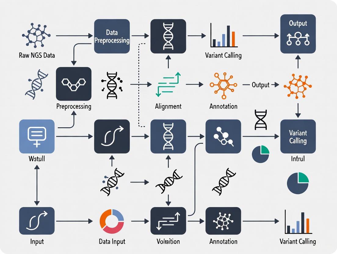
Workflow Visualization
NGS Immunology Data Analysis Flow
Single-Cell Barcoding Concept
FAQs: Troubleshooting Common NGS Bottlenecks
Data Storage and Management
Q: Our data storage costs are escalating rapidly with increasing sequencing volume. What are the key strategies for cost-effective data management? A: Effective data management requires a multi-layered approach. First, implement data lifecycle policies to archive or remove raw data after secondary analysis, as the sheer volume of multiomic data is a primary cost driver [9]. Second, leverage cloud-based systems for scalable storage and high-performance computing, which help address data bottlenecks and enable efficient data sharing [10]. For large-scale initiatives, adopting standardized data formats like those from the Global Alliance for Genomics and Health (GA4GH) improves interoperability and reduces storage complexity [11].
Q: How can we ensure our genomic data is FAIR (Findable, Accessible, Interoperable, and Reusable)? A: Adhering to the FAIR principles requires thorough documentation of all data processing steps and consistent use of version control for both data and code. Utilizing electronic lab notebooks and workflow management systems like Nextflow or Snakemake helps automatically capture these details, ensuring reproducibility and proper data stewardship [11].
Sequencing Errors and Quality Control
Q: A high proportion of our NGS reads contain ambiguities. How should we handle this data for reliable clinical interpretation? A: The optimal strategy depends on the error pattern. For random, non-systematic errors, the neglection strategy (removing sequences with ambiguities) often provides the most reliable prediction outcome [12]. However, if a large fraction of reads contains errors, potentially introducing bias, the deconvolution strategy with a majority vote is preferable, despite being computationally more expensive. Research indicates that the worst-case assumption strategy generally performs worse than both other methods and can lead to overly conservative clinical decisions [12].
Q: Our NGS runs are showing low library yields. What are the most common causes and solutions? A: Low library yield is frequently traced to issues in the pre-analytical phase. The table below outlines common causes and corrective actions [13].
| Cause | Mechanism of Yield Loss | Corrective Action |
|---|---|---|
| Poor Input Quality | Enzyme inhibition from contaminants (salts, phenol) | Re-purify input sample; ensure wash buffers are fresh; target high purity (260/230 > 1.8). |
| Inaccurate Quantification | Suboptimal enzyme stoichiometry from pipetting errors | Use fluorometric methods (Qubit) over UV; calibrate pipettes; use master mixes. |
| Fragmentation Issues | Over-/under-fragmentation reduces adapter ligation efficiency | Optimize fragmentation parameters (time, energy); verify fragmentation profile. |
| Suboptimal Ligation | Poor ligase performance or wrong adapter-to-insert ratio | Titrate adapter:insert ratios; ensure fresh ligase and buffer; maintain optimal temperature. |
Q: What is the typical failure rate for NGS in rare tumor samples, and how do different assays compare? A: A 2025 study on rare tumors found that 14.7% of NGS tests failed due to insufficient quantity or quality of material, affecting 4.7% of patients [14]. The assay type significantly impacted the failure rate. Whole Exome/Transcriptome Sequencing (WETS) was associated with a significantly higher probability of failure compared to smaller targeted panels (Odds Ratio: 11.4). The good news is that repeated testing was successful in 7 out of 8 patients, offering a path to recover from initial failure [14].
Bioinformatics Workflows
Q: Our bioinformatics pipelines are slow, not reproducible, and costly to run. When and how should we optimize them? A: Optimization should begin when usage scales justify the investment, potentially saving 30-75% in time and costs [15]. The process can be broken into three stages:
- Analysis Tools: Identify and implement improved tools, focusing first on the most demanding or unstable points in your pipeline [15].
- Workflow Orchestrator: Introduce a dynamic resource allocation system (e.g., Nextflow) to prevent over-provisioning and reduce computational costs [15].
- Execution Environment: Ensure your compute environment (especially cloud configurations) is cost-optimized to avoid unnecessary expenses [15].
Q: How can automation improve our NGS workflow? A: Integrating automation at various stages enhances consistency and reproducibility. In wet-lab steps, automated pipetting and sample handling reduce human error in DNA/RNA extraction and library preparation [10]. In computational analysis, automation enables features like automatic pipeline triggers upon data arrival, periodic runs, and version tracking, which significantly reduce manual intervention and improve reproducibility [15].
Troubleshooting Guides
Guide 1: Diagnosing and Resolving Data Quality Issues
The "Garbage In, Garbage Out" (GIGO) principle is critical in bioinformatics; poor input data quality inevitably leads to misleading results [11]. Follow this systematic diagnostic flow:
NGS Data Quality Diagnostic Flow
Recommended Error Handling Strategies for Ambiguous Bases: Based on a comparative study, the choice of error handling strategy directly impacts the reliability of clinical predictions [12].
| Strategy | Description | Best For | Performance Note |
|---|---|---|---|
| Neglection | Removes all sequences containing ambiguities (N's). | Scenarios with random, non-systematic errors. | Outperforms other strategies when no systematic errors are present. |
| Deconvolution (Majority Vote) | Resolves ambiguities into all possible sequences; the majority prediction is accepted. | Cases with a high fraction of ambiguous reads or suspected systematic errors. | Computationally expensive but avoids bias from data loss; better than worst-case. |
| Worst-Case Assumption | Always assumes the ambiguity represents the nucleotide worst for therapy (e.g., resistance). | Generally not recommended. | Performance is worse than both neglection and deconvolution strategies. |
Guide 2: Optimizing and Scaling Bioinformatics Workflows
For labs experiencing growing computational demands, migrating to modern, scalable workflow orchestrators is key. A case study with Genomics England successfully transitioned to Nextflow-based pipelines to process 300,000 whole-genome sequencing samples, demonstrating the feasibility of large-scale optimization [15].
Bioinformatics Workflow Optimization Roadmap
The Scientist's Toolkit: Essential Research Reagent Solutions
| Reagent / Material | Function | Key Consideration |
|---|---|---|
| Fluorometric Assay Kits (Qubit) | Accurate quantification of usable nucleic acid concentration, specific to DNA or RNA. | Prefer over UV absorbance (NanoDrop) which can overestimate by counting contaminants [13]. |
| High-Fidelity Polymerase | Amplifies library fragments with minimal introduction of errors during PCR. | Essential for maintaining sequence accuracy; minimizes amplification bias [13]. |
| Magnetic Beads (SPRI) | Purifies and size-selects nucleic acid fragments after enzymatic reactions (e.g., fragmentation, ligation). | Incorrect bead-to-sample ratio is a common pitfall, leading to size selection failures or sample loss [13]. |
| Platform-Specific Adapters | Allows DNA fragments to bind to the sequencing platform and be amplified. | Adapter-to-insert molar ratio must be optimized; excess adapters promote adapter-dimer formation [13] [16]. |
| Fragmentation Enzymes | Shears DNA into uniformly-sized fragments suitable for sequencing. | Over- or under-shearing reduces ligation efficiency and compromises library complexity [13]. |
FAQs and Troubleshooting Guides
▸ FAQ 1: How do data quality and error profiles differ between Illumina and Ion Torrent, and what is the impact on immunology data?
The fundamental difference in sequencing chemistry between the two platforms leads to distinct error profiles that can significantly impact the analysis of immunology data, such as T-cell receptor (TCR) or B-cell receptor (BCR) sequencing.
Answer: Illumina and Ion Torrent technologies employ different detection methods: Illumina uses optical detection of fluorescence signals, while Ion Torrent detects pH changes using semiconductor technology [17]. This fundamental difference results in distinct error profiles.
Illumina sequencing is characterized by high base-call accuracy, with the majority of bases scoring Q30 and above, representing a 99.9% base call accuracy [18]. This high fidelity is crucial for detecting rare clonotypes in immune repertoire sequencing.
In contrast, Ion Torrent sequencing is prone to homopolymer errors (insertions and deletions), though it typically offers longer read lengths and shorter run times [17]. These homopolymer errors can cause frameshifts during translation in gene-based analyses, which is particularly problematic for immunology applications that rely on accurate V(D)J segment identification.
The following table summarizes the key technical differences and their implications for immunology applications:
Table 1: Platform Comparison and Impact on Immunology Data
| Feature | Illumina | Ion Torrent | Impact on Immunology Applications |
|---|---|---|---|
| Chemistry | Optical (fluorescence) [17] | Semiconductor (pH change) [17] | - |
| Primary Error Type | Substitution errors [18] | Homopolymer indels [17] | Frameshifts disrupt CDR3 translation and clonotype assignment. |
| Typical Read Length | Shorter (e.g., 2x150 bp, 2x300 bp) [17] | Longer reads [17] | Advantageous for covering full-length antibody genes. |
| Run Time | Generally longer [17] | Shorter [17] | Faster turnaround for time-sensitive studies. |
| Ideal for Immunology | High-fidelity clonotype tracking, minimal frameshift artifacts. | Targeted panels with frameshift filtering; requires careful data handling. | - |
▸ FAQ 2: My cgMLST analysis from mixed platform data shows inconsistent clustering. What is the cause and how can I resolve it?
Inconsistent clustering in core genome multilocus sequence typing (cgMLST) is a known challenge when integrating data from different sequencing platforms. The root cause often lies in the technology-specific error profiles.
Answer: A study on Listeria monocytogenes directly compared cgMLST results from Illumina and Ion Torrent data. It found that for the same strain, the average allele discrepancy between platforms was 14.5 alleles, which is well above the commonly used threshold of ≤7 alleles for cluster detection in outbreak investigations [17]. This incompatibility can lead to both false-positive and false-negative clusters in immunology studies, such as tracking pathogen-specific immune responses.
Primary Cause: Homopolymer errors in Ion Torrent data lead to frameshift mutations, which cause premature stop codons or altered gene lengths. This results in alleles being called as different when they are, in fact, identical [17].
Solution: Apply a frameshift filter during cgMLST analysis.
- Relative Frameshift Filter (f.s.r.): Removes alleles if their length deviates by a relative fraction (e.g., 0.1) from the median length of all alleles for that locus [17].
- Absolute Frameshift Filter (f.s.a.): Removes alleles if their length deviates by an absolute number of base pairs (e.g., 9 bp) from the median [17].
Applying a strict frameshift filter can reduce the mean allele discrepancy below the 7-allele threshold, improving cluster concordance, though it may slightly reduce discriminatory power [17].
▸ FAQ 3: What are the best practices for designing experiments that combine data from both platforms?
Successfully integrating data from Illumina and Ion Torrent requires careful planning from the experimental design stage through to bioinformatic analysis.
Answer: To ensure compatibility and data quality in mixed-platform immunology studies, follow these best practices:
- Standardize Wet-Lab Protocols: Implement standardized protocols for sample preparation, library construction, and quality control across all participating labs to minimize technical variability [19].
- Use a Common DNA Source: Where possible, use a common source of high-quality DNA for sequencing on different platforms to isolate technology-specific effects from biological variation [17].
- Select the Right Assembler: Not all assemblers handle data from both platforms equally well. The study on L. monocytogenes found that SPAdes was the only assembler that delivered qualitatively comparable results for both Illumina and Ion Torrent data [17].
- Prioritize SNP Analysis for Integration: If your immunology question allows, consider using read-based single nucleotide polymorphism (SNP) analysis. The same study found that the impact of the sequencing platform on SNP analysis was lower than its impact on cgMLST [17].
- Implement Frameshift Filtering: As noted in FAQ 2, always apply frameshift filters to cgMLST data derived from Ion Torrent or mixed-platform studies [17].
- Utilize Positive Controls: Spike in a known control (e.g., 20% PhiX for Illumina) during sequencing to act as a positive control for clustering and to monitor run quality [20].
▸ FAQ 4: How can I troubleshoot a complete sequencing failure, such as a "Cycle 1" error on my MiSeq?
A "Cycle 1" error indicates a fundamental failure in the initial phase of the sequencing run, where the instrument cannot find sufficient signal to focus.
Answer: "Cycle 1" errors on an Illumina MiSeq (with error messages like "Best focus not found" or "No usable signal found") can be due to library, reagent, or instrument issues [20]. Follow this systematic troubleshooting workflow to diagnose and resolve the problem.
Diagram 1: MiSeq Cycle 1 Error Troubleshooting Workflow
Key Investigation Steps for Library and Reagents:
- Reagent Kits: Check for expiration dates and ensure proper storage conditions [20].
- Library Quality: Verify the quality and quantity of your library using Illumina-recommended fluorometric methods (e.g., Qubit) – do not rely solely on absorbance (NanoDrop) [13] [20].
- Library Design: Ensure your library design, including any custom primers (common in immunology panels), is compatible with the Illumina platform [20].
- NaOH Dilution: Confirm that a fresh dilution of NaOH was used for denaturation and that its pH is above 12.5 [20].
▸ FAQ 5: My library yield is low. What are the common causes and how can I improve it?
Low library yield is a frequent bottleneck that can derail NGS projects. The causes can be traced to several steps in the preparation process.
Answer: Low final library yield can result from issues at multiple stages. The table below outlines common root causes and their corrective actions.
Table 2: Troubleshooting Low NGS Library Yield
| Root Cause | Mechanism of Yield Loss | Corrective Action |
|---|---|---|
| Poor Input Quality | Enzyme inhibition from contaminants (phenol, salts, EDTA) or degraded DNA/RNA [13]. | Re-purify input sample; ensure high purity (260/230 > 1.8); use fluorometric quantification (Qubit) [13]. |
| Fragmentation Issues | Over- or under-fragmentation produces fragments outside the optimal size range for adapter ligation [13]. | Optimize fragmentation parameters (time, energy); verify fragment size distribution post-shearing. |
| Suboptimal Adapter Ligation | Poor ligase performance or incorrect adapter-to-insert molar ratio reduces library molecule formation [13]. | Titrate adapter:insert ratio; use fresh ligase and buffer; ensure optimal reaction temperature. |
| Overly Aggressive Cleanup | Desired fragments are accidentally removed during bead-based purification or size selection [13]. | Precisely follow bead-to-sample ratios; avoid over-drying beads; use validated cleanup protocols. |
▸ Computational Considerations for Large-Scale NGS Immunology Data
Framing the aforementioned challenges within the context of solving computational bottlenecks requires a holistic strategy that extends from the sequencer to the analysis software.
1. Leverage AI-Powered Tools: The field is shifting towards AI-based bioinformatics tools that can increase analysis accuracy by up to 30% while cutting processing time in half [21]. Tools like DeepVariant use deep learning for more accurate variant calling, which is critical for identifying somatic hypermutations in immunoglobulins [22] [21].
2. Adopt Cloud Computing: The massive volume of data from mixed-platform studies often exceeds local computational capacity. Cloud platforms (AWS, Google Cloud Genomics) provide scalable infrastructure, enable global collaboration, and are cost-effective for smaller labs [22]. They also implement stringent security protocols compliant with HIPAA and GDPR [22].
3. Implement Standardized Pipelines: Reproducibility is a major challenge when integrating diverse datasets. Adopt community-validated workflows for preprocessing, normalization, and analysis [19]. For immune repertoire analysis, using standardized tools like MiXCR—a gold-standard tool used in 47 of the top 50 research institutions—ensures consistency and accuracy across projects and platforms [19].
Diagram 2: Computational Pipeline for Multi-Platform Immunology Data
▸ The Scientist's Toolkit: Key Research Reagent Solutions
Table 3: Essential Materials and Tools for NGS Immunology Workflows
| Item / Tool | Function | Relevance to Immunology & Platform Challenges |
|---|---|---|
| SPAdes Assembler | Genome assembly from sequencing reads. | Crucial for generating comparable assemblies from both Illumina and Ion Torrent data [17]. |
| Frameshift Filters (f.s.r., f.s.a.) | Bioinformatic filters for cgMLST analysis. | Mitigates homopolymer errors from Ion Torrent data, enabling integration with Illumina datasets [17]. |
| PhiX Control Library | Sequencing run quality control. | Serves as a positive control to diagnose platform-specific issues (e.g., "Cycle 1" errors) [20]. |
| Fluorometric Quantifier (e.g., Qubit) | Accurate quantification of DNA/RNA. | Prevents low yield and failed libraries by measuring only usable nucleic acids, not contaminants [13]. |
| MiXCR Software | Specialized tool for immune repertoire analysis. | Provides a standardized, high-performance pipeline for analyzing TCR and BCR sequencing data [19]. |
| Illumina DNA Prep Kit | Library preparation for Illumina platforms. | Standardized, high-quality library construction to minimize prep-related bias [17]. |
| Ion Plus Fragment Library Kit | Library preparation for Ion Torrent platforms. | Optimized library construction for semiconductor sequencing [17]. |
In large-scale NGS immunology research, the boundary between laboratory preparation and computational analysis is not just crossed frequently—it is a major site of operational friction. Errors introduced during library preparation do not merely compromise sample quality; they actively distort downstream bioinformatics processes, exacerbating computational bottlenecks and consuming precious processing time, storage, and financial resources [23] [24].
This guide addresses the critical interplay between library preparation and computational load, providing targeted troubleshooting to help researchers and drug development professionals produce cleaner data, ensure more efficient analysis, and accelerate discovery.
Troubleshooting FAQs: From Library Prep Error to Computational Symptom
FAQ 1: My sequencing run finished, but the variant caller reported extremely high duplicate reads and poor genome coverage. What went wrong in library prep?
- Problem: High duplication rates and flat coverage are classic computational symptoms of low library complexity, meaning an insufficient number of unique DNA fragments were sequenced.
- Primary Library Prep Cause: This is frequently caused by low input DNA/RNA, degraded starting material, or overly aggressive PCR amplification during library construction [13]. Poor input quality forces the sequencer to repeatedly read the same limited set of fragments.
- Computational Impact: Variant callers like GATK and FreeBayes waste significant processing power analyzing duplicate reads, which provide no new biological information and increase false positive rates [25] [26]. This leads to longer compute times and unreliable results.
- Solution:
- Verify Input Quality: Use fluorometric quantification (e.g., Qubit) over UV absorbance to ensure accurate measurement of amplifiable DNA. Check RNA Integrity Numbers (RIN) for RNA-seq.
- Limit PCR Cycles: Use the minimum number of PCR cycles necessary for library amplification. If yield is low, it is better to repeat the amplification than to add excessive cycles [27] [13].
- Assess Post-Ligation Yield: Check library yield after the ligation step, before PCR, to identify if amplification is masking an underlying inefficiency.
FAQ 2: My data analysis reveals a high percentage of reads that won't align to the reference genome. What is the likely culprit?
- Problem: A low alignment rate in tools like BWA or HISAT2 indicates a large proportion of sequences are not part of the target genome [26].
- Primary Library Prep Cause: The most common cause is the presence of adapter dimers—short fragments composed only of adapter sequences that ligate to each other [27] [28] [13]. These non-informative sequences are amplified and sequenced, consuming flow cell space and generating unalignable data.
- Computational Impact: Adapter dimers force the alignment software to process millions of useless reads, drastically increasing analysis time and storage needs for temporary files. They also reduce the usable sequencing depth for the actual experiment.
- Solution:
- Optimize Size Selection: Perform a rigorous bead-based clean-up or gel extraction to remove fragments shorter than your intended insert size. A sharp peak at ~70-90 bp on a Bioanalyzer trace indicates adapter dimers [27] [13].
- Optimize Ligation Conditions: Ensure correct adapter-to-insert molar ratios to prevent adapter self-ligation. Use fresh, properly stored adapters [29].
- Use Trimming Tools: As a last resort, employ preprocessing tools like Cutadapt or Trimmomatic to identify and remove adapter sequences from the raw reads before alignment, though this adds an extra computational step [26].
FAQ 3: I see high variability in read depth across samples in my multiplexed run, forcing me to re-analyze data. How can this be prevented?
- Problem: Inconsistent read depth between samples in a pooled library leads to some targets being over-sequenced and others under-sequenced, compromising statistical power.
- Primary Library Prep Cause: Inaccurate library quantification and normalization prior to pooling. Manual quantification using absorbance methods and pipetting inaccuracies are frequent sources of error [13] [30].
- Computational Impact: Researchers must spend extra time and cloud computing credits to re-pool and re-sequence samples, or apply complex normalization algorithms during differential expression analysis (e.g., in DESeq2), which can introduce bias [26].
- Solution:
- Use qPCR for Quantification: Perform library quantification using qPCR-based kits (e.g., Ion Library Quantitation Kit) as they measure amplifiable molecules, which is what determines cluster generation on the sequencer [27].
- Automate Normalization: Implement automated liquid handling systems to improve pipetting precision and consistency during the normalization and pooling steps [29] [30].
- Use Auto-Normalizing Kits: Consider library prep kits that feature built-in normalization, which can maintain consistent read counts across a wide range of input concentrations [30].
Quantitative Guide: Library Prep Failures and Their Downstream Consequences
The table below summarizes how specific library preparation errors manifest in the data and their direct impact on the computational workflow.
Table 1: Troubleshooting Guide: Library Prep Errors and Downstream Computational Impact
| Library Prep Error | Observed Failure Signal | Downstream Computational Symptom | Corrective Action |
|---|---|---|---|
| Adapter Dimer Formation [27] [13] | Sharp peak at ~70-90 bp on Bioanalyzer; Low alignment rate. | Wasted sequencing cycles; Increased processing time by aligners (BWA, HISAT2); Increased storage for useless data. | Optimize adapter ligation ratios; Implement rigorous bead-based size selection [29]. |
| Low Input/Degraded Sample [13] [30] | Low library yield; High duplication rate reported by tools like Picard. | Variant callers (GATK) process redundant data; Reduced statistical power; Increased false positives/negatives. | Verify input quality with fluorometry (Qubit); Use minimum required input DNA/RNA. |
| Over-amplification in PCR [13] | High duplication rate; Skewed fragment size distribution. | Increased computational burden in duplicate marking; Bias in variant calling and expression quantification. | Reduce the number of PCR cycles; Optimize amplification from ligation product [27]. |
| Inaccurate Library Normalization [30] | Uneven read depth across samples in a multiplexed run. | Requires re-sequencing or computational normalization in analysis (e.g., DESeq2), consuming extra time and cloud compute resources. | Use qPCR for quantification; Automate pooling with liquid handlers [29]. |
| Sample Contamination [30] | Presence of unexpected species or sequences in taxonomic profiling. | Complicates metagenomic analysis (Kraken, MetaPhlAn); Leads to misinterpretation of results and wasted analysis. | Use sterile techniques; Include negative controls; Re-purify samples with clean columns/beads [13]. |
The Scientist's Toolkit: Essential Reagents and Computational Links
The following reagents and tools are critical for preventing the errors discussed above and ensuring a smooth transition to computational analysis.
Table 2: Research Reagent Solutions and Their Functions
| Item | Function in Library Prep | Role in Mitigating Computational Load |
|---|---|---|
| Fluorometric Quantification Kits (e.g., Qubit) [13] | Accurately measures concentration of amplifiable nucleic acids, unlike UV absorbance. | Prevents low-complexity libraries, reducing duplicate reads and saving variant calling computation. |
| qPCR-based Library Quant Kits [27] | Precisely quantifies "amplifiable" library molecules before pooling. | Ensures even read depth across samples, avoiding the need for re-sequencing or complex data normalization. |
| High-Fidelity DNA Polymerase | Reduces errors during PCR amplification and enables fewer cycles. | Minimizes introduction of sequencing artifacts that must be filtered out during bioinformatic processing. |
| Robust Size Selection Beads [13] | Efficiently removes adapter dimers and selects for the desired insert size range. | Prevents generation of unalignable reads, streamlining the alignment process and improving usable data yield. |
| Automated Liquid Handlers (e.g., I.DOT) [29] [30] | Eliminates pipetting inaccuracies and variability in repetitive steps. | Reduces batch effects and normalization errors, leading to cleaner data that requires less corrective computation. |
Visual Workflow: How Library Prep Choices Ripple Through Data Analysis
The diagram below illustrates the cascading effect of library preparation quality on downstream computational processes, highlighting key bottlenecks.
Library Prep to Compute Impact Flow
In the context of large-scale NGS immunology research, the path to solving computational bottlenecks does not begin with more powerful servers or faster algorithms alone. It starts at the laboratory bench. By recognizing library preparation as the foundational step that dictates data quality, researchers can make strategic investments—in optimized protocols, precise quantification, and automation—that pay substantial dividends in computational efficiency [29] [30].
A disciplined approach to library prep reduces wasted sequencing cycles, minimizes the need for complex data correction, and ensures that the powerful computational tools for variant calling, differential expression, and metagenomic analysis are operating on the cleanest possible data. This synergy between wet-lab practice and dry-lab analysis is the key to accelerating drug development and unlocking meaningful biological insights from immunogenomic data.
Technical Support Center
HLA Typing: Troubleshooting & FAQs
Q1: My HLA typing results from NGS data show low coverage for certain exons. What could be the cause and how can I resolve it?
A: Low coverage in specific exons, particularly in HLA Class II genes, is a common computational bottleneck. This is often due to high sequence similarity between HLA alleles and the presence of intronic regions.
- Cause: Misalignment of sequencing reads to the incorrect reference genome or a reference that lacks comprehensive HLA allele diversity.
- Solution:
- Use an HLA-Optimized Aligner: Switch from a general-purpose aligner (like BWA) to a specialized tool (e.g.,
HLAminer,Kourami,OptiType). These tools use a graph-based or allele-specific approach to handle high polymorphism. - Employ an HLA-Enhanced Reference: Use a reference panel that includes a wide array of known HLA sequences (e.g., the IPD-IMGT/HLA database) to improve mapping accuracy.
- Check Primer Binding Sites: If using amplicon-based sequencing, validate that your primer sequences are not overlapping with known polymorphisms that could cause amplification bias.
- Use an HLA-Optimized Aligner: Switch from a general-purpose aligner (like BWA) to a specialized tool (e.g.,
Q2: How do I interpret the ambiguity in my HLA typing output, such as a result listed as "HLA-A*02:01:01G"?"
A: Ambiguity arises when different combinations of polymorphisms across the gene yield identical sequencing reads for the exons tested.
- Interpretation: "G" groups (e.g.,
*02:01:01G) represent alleles that are identical in their peptide-binding regions (exons 2 and 3 for Class I; exon 2 for Class II). For most functional studies, this level of resolution is sufficient. - Resolution: To resolve "field" ambiguities (e.g.,
*02:01vs*02:05), you need:- Wet-Lab: Phase-separated sequencing (e.g., long-read sequencing) to determine which polymorphisms are on the same chromosome.
- In-Silico: Use computational phasing tools that leverage read-pair information or population-based haplotype frequencies.
Experimental Protocol: High-Resolution HLA Typing from Whole Genome Sequencing (WGS) Data
- Data Input: Paired-end WGS reads (FASTQ format).
- Quality Control: Use
FastQCandTrimmomaticto assess and trim adapter sequences and low-quality bases. - Alignment & Typing:
- Execute
Kouramiwith its bundled HLA reference graph. - Command:
java -jar Kourami.jar -r <reference_dir> -s <sample_id> -o <output_dir> <input_bam_file>
- Execute
- Result Interpretation: The output provides the most likely 4-digit (or higher) HLA alleles. Cross-reference the reported alleles with the IPD-IMGT/HLA database for functional annotation.
HLA Typing from WGS Data
TCR/BCR Repertoire: Troubleshooting & FAQs
Q1: My TCR/BCR repertoire analysis shows a very low diversity index. Is this a technical artifact or a true biological signal?
A: It can be either. Systematic errors must be ruled out before biological interpretation.
Technical Causes & Solutions:
- Low Input DNA/RNA: Increases stochastic PCR bias. Use a quantitative method (e.g., Qubit, Bioanalyzer) to ensure sufficient starting material.
- PCR Over-Amplification: Leads to dominance by a few high-abundance clones. Optimize PCR cycle number and use unique molecular identifiers (UMIs) to correct for amplification bias.
- Bioinformatic Preprocessing: Inadequate quality filtering or primer trimming can remove valid reads. Re-inspect raw read quality and adjust preprocessing parameters.
Biological Signal: A low diversity index is a valid finding in contexts like acute immune response, immunosenescence, or certain immunodeficiencies.
Q2: How can I accurately track the same T-cell or B-cell clone across multiple time points or tissues?
A: This requires high-specificity clonotype tracking.
- Method: Use the CDR3 nucleotide sequence as the clone identifier, as it is the most specific marker.
- Computational Protocol:
- UMI Deduplication: For each sample, group reads by UMI and assemble a consensus CDR3 sequence to eliminate PCR and sequencing errors.
- Clonotype Definition: Define clonotypes based on identical CDR3 amino acid sequences and V/J gene assignments.
- Cross-Sample Comparison: Use a tool like
alakazamorscRepertoire(for single-cell data) to calculate clonotype overlap and abundance across samples.
Experimental Protocol: TCRβ Repertoire Sequencing with UMIs
- Library Prep: Use a multiplex PCR system (e.g., Adaptive Biotechnologies' ImmunoSEQ, iRepertoire) with primers containing UMIs.
- Sequencing: High-throughput sequencing on an Illumina platform (2x150bp or 2x250bp recommended).
- Bioinformatic Processing:
- UMI Extraction & Error Correction: Use
pRESTOorMiGECto group reads by UMI and generate consensus sequences. - V(D)J Assignment: Align consensus sequences to a V(D)J reference using
IgBLASTorMiXCR. - Clonotype Table Generation: Collapse identical CDR3aa + V + J combinations to create a frequency table.
- UMI Extraction & Error Correction: Use
TCR Rep Sequencing with UMIs
V(D)J Analysis: Troubleshooting & FAQs
Q1: My V(D)J rearrangement analysis from single-cell RNA-seq data has a low cell recovery rate. What are the key parameters to check?
A: Low cell recovery is often due to suboptimal data processing.
- Key Parameters:
- Cell Barcodes: Ensure the correct barcode whitelist and barcode length are specified. Low-quality bases at the start of Read 1 can cause barcode misidentification.
- Read Orientation: Confirm that the sequence of the constant region primer is correctly specified and that the tool is searching for it on the correct strand.
- Alignment Confidence: Increase the
--expect-cellsparameter inCell Ranger vdjif you loaded more cells than the default (e.g., 10,000), or adjust the alignment scoring thresholds in other tools.
Q2: How can I visualize the clonal relationships and somatic hypermutation (SHM) in my B-cell data?
A: This requires constructing lineage trees.
- Method:
- Data Extraction: For a clone of interest, extract all heavy-chain sequences (germline-aligned VDJ sequences and their UMIs/counts).
- Germline Reconstruction: Infer the unmutated common ancestor sequence using a tool like
IgPhyMLorpartis. - Tree Building: Input the germline sequence and the mutated sequences into a phylogenetic tree builder (e.g,
PHYLIP,dnaml) that can handle high mutation rates.
Experimental Protocol: Single-Cell V(D)J and Gene Expression Analysis (10x Genomics)
- Library Preparation: Generate both 5' Gene Expression and V(D)J libraries from the same single-cell suspension following the manufacturer's protocol.
- Sequencing: Sequence libraries on an Illumina NovaSeq or HiSeq.
- Data Processing:
- Run
Cell Ranger multito simultaneously analyze both libraries, using the--feature-reffile to link the two datasets. - This produces a unified feature-barcode matrix containing clonotype information for each cell barcode.
- Run
- Downstream Analysis: In R, use the
SeuratandscRepertoirepackages to integrate clonality with cluster phenotypes and perform trajectory analysis on expanded clones.
Single-Cell V(D)J + GEX Workflow
Table 1: Comparison of HLA Typing Tools (Theoretical Performance on WGS Data)
| Tool | Algorithm Type | Required Read Length | Reported 4-Digit Accuracy | Key Computational Bottleneck |
|---|---|---|---|---|
| Kourami | Graph-based alignment | >= 100bp | >99% | High memory usage for graph construction |
| OptiType | Integer Linear Programming | >= 50bp | >97% | Limited to HLA Class I genes |
| HLAminer | Read alignment & assembly | >= 150bp | >95% | Long runtime for assembly step |
| PolySolver | Bayesian inference | >= 100bp | >96% | Sensitivity to alignment errors |
Table 2: Key Metrics for TCR Repertoire Quality Control
| Metric | Acceptable Range | Indication of Problem |
|---|---|---|
| Reads per Clone | Even distribution, long tail | A few clones with extremely high counts indicate PCR bias. |
| Clonotype Diversity (Shannon) | Context-dependent | Very low diversity may indicate technical bottlenecking. |
| UMI Saturation | >80% | Lower values suggest insufficient sequencing depth. |
| In-Frame Rearrangements | >85% of productive clones | Lower rates suggest poor RNA quality or bioinformatic errors. |
The Scientist's Toolkit
Table 3: Essential Reagents & Tools for NGS Immunology
| Item | Function | Example Product/Software |
|---|---|---|
| UMI Adapters | Tags each original molecule with a unique barcode to correct for PCR and sequencing errors. | NEBNext Multiplex Oligos for Illumina |
| Multiplex PCR Primers | Amplifies all possible V(D)J rearrangements in a single reaction from bulk cells. | iRepertoire Human TCR/BCR Primer Sets |
| Single-Cell Barcoding Kit | Labels cDNA from individual cells with a unique barcode for cell-specific V(D)J recovery. | 10x Genomics Single Cell 5' Kit |
| HLA Allele Database | Reference set for accurate alignment and typing of highly polymorphic HLA genes. | IPD-IMGT/HLA Database |
| V(D)J Reference Set | Curated database of germline V, D, and J gene segments for alignment. | IMGT Reference Directory |
| Specialized Aligner | Software optimized for resolving complex, hypervariable immune sequences. | MiXCR, IgBLAST |
Advanced Computational Methods for NGS Immunology Data
Machine Learning Integration for Multimodal Immunological Data
Next-Generation Sequencing (NGS) has revolutionized immunology research by enabling high-throughput analysis of immune repertoires, cell states, and functions. However, the integration of multimodal immunological data—spanning genomics, transcriptomics, proteomics, and clinical information—presents significant computational challenges that form the central bottleneck in large-scale NGS immunology research. The convergence of artificial intelligence (AI) with NGS technologies offers transformative potential to overcome these hurdles, accelerating the pace from data generation to biological insight and clinical application [31] [32].
This technical support center addresses the specific computational and methodological challenges researchers encounter when implementing machine learning for multimodal immunological data analysis. The guidance provided is framed within the broader thesis that strategic computational approaches can effectively resolve these bottlenecks, enabling robust, reproducible, and clinically actionable findings in immunology.
Troubleshooting Guides: Resolving Critical Bottlenecks
Data Quality and Preprocessing Issues
Problem: Sequencing Errors and Quality Control Failures Sequencing errors in NGS data can introduce false variants and significantly impact downstream ML model performance. In immunology, this is particularly critical when analyzing B-cell or T-cell receptor repertoires where single nucleotide variations can alter receptor specificity [1].
Solutions:
- Implement Robust QC Pipelines: Use tools like FastQC and MultiQC for comprehensive quality assessment. Establish strict quality thresholds based on your specific immunological application.
- AI-Enhanced Error Correction: Employ ML tools like DeepVariant which uses deep learning to distinguish true genetic variants from sequencing errors, significantly improving accuracy over traditional methods [31] [32].
- Batch Effect Correction: Utilize combat-like algorithms or neural network approaches (e.g., VAEs) to remove technical artifacts while preserving biological signals, especially crucial when integrating data from multiple experiments or time points.
Table 1: Quality Control Metrics and Thresholds for NGS Immunology Data
| Metric | Optimal Range | Threshold for Concern | Corrective Action |
|---|---|---|---|
| Phred Quality Score | ≥Q30 for >80% bases | Trimming, filtering, or resequencing | |
| Read Depth (Immunology Panels) | 500-1000x | <200x | Increase sequencing depth |
| Duplication Rate | <10-20% | >50% | Optimize library preparation |
| Base Balance | Even across cycles | Significant bias | Check sequencing chemistry |
Problem: Data Heterogeneity and Integration Challenges Multimodal immunology data often comes from diverse sources—genomic, transcriptomic, proteomic, and clinical—each with different scales, distributions, and missing data patterns [33] [34].
Solutions:
- Cross-Modal Imputation: Use neural network architectures (e.g., autoencoders) specifically designed for imputing missing data across modalities while preserving biological relationships.
- Harmonization Techniques: Implement MNN (Mutual Nearest Neighbors) or deep learning-based alignment methods when integrating datasets from different batches, technologies, or institutions.
- Feature Standardization: Apply modality-specific normalization (e.g., CPM for RNA-seq, arcsinh for CyTOF) before integration to maintain technical consistency.
Model Training and Performance Issues
Problem: Poor Model Generalization Despite High Training Accuracy Immunology datasets often suffer from high dimensionality with relatively small sample sizes, leading to overfitting despite apparent good performance during training [35] [36].
Solutions:
- Regularization Strategies: Implement L1/L2 regularization, dropout in neural networks, or ensemble methods like Random Forests which are naturally robust to overfitting.
- Cross-Validation Protocols: Use nested cross-validation with appropriate stratification to account for cohort effects in immunological studies.
- Data Augmentation: For image-based immunology data (e.g., histopathology), employ rotation, flipping, and color variations. For sequence data, consider synthetic minority oversampling or generative adversarial networks (GANs) to create realistic synthetic data [32].
Problem: Model Interpretability Barriers in Clinical Translation The "black box" nature of complex ML models hinders clinical adoption in immunology, where understanding biological mechanisms is as important as prediction accuracy [33] [37].
Solutions:
- Explainable AI (XAI) Techniques: Implement SHAP (SHapley Additive exPlanations) or LIME (Local Interpretable Model-agnostic Explanations) to quantify feature importance.
- Attention Mechanisms: Use transformer models with built-in attention layers that can highlight relevant sequence regions or cell populations driving predictions.
- Biological Validation: Always correlate ML-derived features with known immunological pathways and validate findings through experimental follow-up.
Table 2: Performance Benchmarks for ML Models on Immunology Tasks
| Model Type | Typical Accuracy Range | Best For Immunology Use Cases | Interpretability |
|---|---|---|---|
| Random Forest | 75-92% | Patient stratification, biomarker discovery | Medium (feature importance) |
| XGBoost | 78-95% | Treatment response prediction | Medium (feature importance) |
| Neural Networks | 82-97% | Image analysis, sequence modeling | Low (requires XAI) |
| Transformer Models | 85-98% | Immune repertoire analysis | Medium (attention weights) |
Computational Infrastructure Limitations
Problem: Processing Delays with Large-Scale Immunology Datasets Multimodal immunology datasets, especially single-cell and spatial transcriptomics, can reach terabytes in scale, overwhelming conventional computational resources [1] [32].
Solutions:
- Federated Learning: Implement privacy-preserving distributed ML approaches that train models across multiple institutions without sharing raw patient data, crucial for multi-center immunology studies [31].
- Cloud and HPC Utilization: Leverage GPU acceleration (NVIDIA Parabricks) which can accelerate genomic analyses by up to 80x compared to CPU-based workflows [32].
- Progressive Analysis: Implement stochastic gradient methods that process data in mini-batches rather than loading entire datasets into memory.
Frequently Asked Questions (FAQs)
Q1: What machine learning approach works best for integrating genomic, transcriptomic, and proteomic data in immunology studies?
Multimodal AI approaches that combine multiple data types consistently outperform single-data models, showing an average 6.4% increase in predictive accuracy [38]. The optimal architecture depends on your specific research question:
- Early Fusion: Combine raw data from multiple modalities before feature extraction when modalities are highly correlated.
- Intermediate Fusion: Use separate feature extractors for each modality with a shared integration layer (e.g., multimodal autoencoders).
- Late Fusion: Train separate models on each modality and combine predictions, ideal when modalities have different statistical properties.
For immunology applications, intermediate fusion with dedicated neural network encoders for each data type typically performs best, allowing the model to learn both modality-specific and cross-modal representations [33] [34].
Q2: How can we address the 'small n, large p' problem in immunological datasets where we have many more features than samples?
This high-dimensionality challenge is common in immunology research. Several strategies have proven effective:
- Dimensionality Reduction: Use UMAP or t-SNE for visualization, but employ PCA or autoencoders for feature reduction before model training.
- Feature Selection: Prioritize biologically informed feature selection (e.g., known immune pathways) before applying ML, or use regularized models (Lasso, Elastic Net) that perform implicit feature selection.
- Transfer Learning: Leverage pre-trained models on larger public datasets (e.g., ImmPort, TCGA) and fine-tune on your specific immunology dataset [36].
- Data Augmentation: Carefully apply synthetic data generation techniques, particularly for immune repertoire sequencing data where legitimate sequence variations can be modeled.
Q3: What are the best practices for validating ML models in immunology to ensure findings are biologically meaningful and reproducible?
Robust validation is crucial for immunological applications:
- External Validation: Always validate models on completely independent cohorts, ideally from different institutions or collected using different protocols.
- Biological Plausibility Check: Ensure model predictions align with established immunological knowledge; use pathway enrichment analysis on important features.
- Experimental Validation: Design flow cytometry, functional assays, or animal models to test key predictions from your ML models.
- Benchmarking: Compare performance against established immunological benchmarks and traditional statistical methods to demonstrate added value [35].
Q4: How can we effectively handle missing data across multiple modalities in immunology datasets?
Missing data is common in multimodal studies. The optimal approach depends on the missingness mechanism:
- ML-Based Imputation: Use sophisticated imputation methods like MICE (Multiple Imputation by Chained Equations) or neural network approaches (GAIN) for data missing at random.
- Model-Level Handling: Employ algorithms like XGBoost that naturally handle missing values, or use mask-based approaches in neural networks.
- Strategic Exclusion: For modalities with >40% missingness, consider excluding that modality entirely rather than relying on highly imputed data.
Q5: What computational resources are typically required for large-scale immunology ML projects?
Requirements vary by project scale:
- Moderate Scale (Single-cell RNA-seq of 10,000-100,000 cells): 16-32 CPU cores, 64-128GB RAM, potential GPU acceleration (NVIDIA V100 or A100).
- Large Scale (Population immunology, millions of cells): High-performance computing clusters, specialized genomic databases, cloud computing solutions with distributed processing capabilities [1] [32].
Table 3: Computational Requirements for Common Immunology ML Tasks
| Analysis Type | Recommended RAM | CPU Cores | GPU | Storage |
|---|---|---|---|---|
| Bulk RNA-seq DE Analysis | 16-32GB | 8-16 | Optional | 50-100GB |
| Single-cell RNA-seq (10k cells) | 32-64GB | 16-32 | Recommended | 100-200GB |
| Immune Repertoire Sequencing | 64-128GB | 16-32 | Highly Recommended | 200-500GB |
| Multimodal Integration (3+ modalities) | 128GB+ | 32+ | Essential | 500GB-1TB+ |
Experimental Protocols for Key Methodologies
Protocol: ML-Driven Immune Response Prediction
Objective: Predict response to immune checkpoint blockade therapy using integrated multimodal data [34].
Materials and Methods:
- Data Collection:
- Collect pre-treatment tumor samples with matched genomic (WES/WGS), transcriptomic (RNA-seq), and clinical data
- Include at least 50 responders and 50 non-responders for statistical power
Feature Engineering:
- Genomic Features: Calculate tumor mutation burden, neoantigen load, specific mutation status (e.g., POLE, POLD1)
- Transcriptomic Features: Compute immune cell scores (using CIBERSORTx), gene expression signatures (IFN-γ, expanded-immune signature)
- Clinical Features: Include PD-L1 expression, tumor stage, previous treatments
Model Training:
- Implement ensemble methods (Random Forest, XGBoost) as baseline
- Compare with neural network architectures specifically designed for multimodal integration
- Use 5-fold cross-validation with stratification by response status
Validation:
- Validate on independent cohort with same data modalities
- Perform permutation testing to assess significance
- Use SHAP analysis to identify most predictive features
Protocol: Automated Variant Reporting in Immunology
Objective: Implement ML-based clinical decision support for variant reporting in immunology-related genes [37].
Materials and Methods:
- Data Curation:
- Collect historical variant calls with expert curation labels (reportable vs. not reportable)
- Include at least 1,000 variants with ground truth classifications
- Extract 200+ features per variant including functional prediction scores, population frequency, conservation scores
Model Development:
- Train tree-based ensemble models (Random Forest, XGBoost) which have shown excellent performance (PRC AUC 0.891-0.995)
- Implement neural networks for comparison
- Address class imbalance using SMOTE or weighted loss functions
Interpretability Implementation:
- Integrate SHAP values or LIME for explainable predictions
- Create waterfall plots showing feature contributions for each variant
- Establish confidence thresholds for automated vs. manual review
Clinical Integration:
- Deploy as part of tertiary analysis platform
- Implement continuous learning from expert feedback
- Maintain audit trail of all automated decisions
Table 4: Key Research Reagent Solutions for ML in Immunology
| Resource Category | Specific Tools/Platforms | Primary Function | Application in Immunology |
|---|---|---|---|
| Sequencing Platforms | Illumina NovaSeq, PacBio Revio, Oxford Nanopore | High-throughput data generation | Immune repertoire sequencing, single-cell immunology |
| Data Analysis Suites | Illumina BaseSpace, DNAnexus, Lifebit | Cloud-based NGS analysis | Multimodal data integration without advanced programming |
| Variant Calling | DeepVariant, GATK, NVIDIA Parabricks | Accurate variant identification | Somatic variant detection in cancer immunology |
| Single-cell Analysis | Cell Ranger, Seurat, Scanpy | Processing single-cell data | Immune cell atlas construction, cell state identification |
| ML Frameworks | TensorFlow, PyTorch, Scikit-learn | Model development and training | Predictive model building for immune responses |
| Immunology-Specific DB | ImmPort, VDJerry, ImmuneCODE | Reference data repositories | Training data for immune-specific models |
| Visualization Tools | UCSC Genome Browser, Cytoscape, UMAP/t-SNE | Data exploration and presentation | Immune repertoire dynamics, cell population visualization |
Advanced Methodologies and Future Directions
Emerging Approaches: Federated Learning for Multi-Center Immunology Studies
Federated learning enables collaborative model training across institutions without sharing sensitive patient data, addressing critical privacy concerns in immunology research [31]. This approach is particularly valuable for:
- Rare Immune Disorders: Pooling knowledge across multiple centers to overcome small sample sizes
- Global Health Immunology: Studying population-specific immune responses while maintaining data sovereignty
- Clinical Trial Optimization: Developing predictive models using data from multiple trial sites without centralizing data
Implementation requires specialized platforms (e.g., Lifebit, NVIDIA FLARE) and careful attention to data harmonization across sites to ensure model robustness.
Third-Generation Sequencing Integration
Long-read sequencing technologies (PacBio, Oxford Nanopore) present new opportunities and challenges for immunological research:
- Complete Immune Receptor Characterization: Sequencing full-length B-cell and T-cell receptors without assembly
- Epigenetic Modifications: Direct detection of methylation patterns in immune cells using Nanopore sequencing
- Integrated Multiomics: Simultaneous measurement of transcriptome and epigenome from the same cell
AI approaches are evolving to handle the unique characteristics of third-generation sequencing data, including higher error rates that require specialized basecalling models and error correction algorithms [31] [9].
Through systematic implementation of these troubleshooting guides, experimental protocols, and computational strategies, researchers can effectively overcome the bottlenecks in large-scale NGS immunology research, accelerating the translation of multimodal data into immunological insights and therapeutic advances.
This technical support center addresses common challenges in analyzing large-scale Next-Generation Sequencing (NGS) data for immunology research. The following guides provide solutions for persistent computational bottlenecks.
Frequently Asked Questions (FAQs)
1. What is the primary purpose of ImmunoDataAnalyzer? ImmunoDataAnalyzer (IMDA) is a bioinformatics pipeline that automates the processing of raw NGS data into analyzable immune repertoires. It covers the entire workflow from initial quality control and clonotype assembly to the comparison of multiple T-cell receptor (TCR) and immunoglobulin (IG) repertoires, facilitating the calculation of clonality, diversity, and V(D)J gene segment usage [39].
2. My analysis pipeline failed with an error about a missing endogenous control. What does this mean? This error typically occurs due to a configuration conflict between singleplex and multiplex experiment data within an analysis group. To resolve it, you can either: a) separate the singleplex and multiplex data into distinct analysis groups, or b) configure the current analysis group to skip target normalization [40].
3. I am seeing a high fraction of cells with zero transcripts in my single-cell data. What could be the cause? An unusually high fraction of empty cells can be caused by two main issues. First, the gene panel used may not contain genes expressed by a major cell type in your sample. Second, it could indicate poor cell segmentation. It is recommended to verify that your gene panel is well-matched to the sample and then use visualization tools to inspect the accuracy of cell boundaries [41].
4. How can I handle the massive computational demands of NGS data analysis? Large datasets from whole-genome or transcriptome studies require powerful, optimized workflows. Proven solutions include using efficient data formats (like Parquet), high-performance tools like MiXCR, and leveraging scalable computational environments like cloud platforms (AWS, GCP, Azure) or high-performance computing (HPC) clusters. User-friendly interfaces are also making these powerful resources more accessible to biologists [2] [1] [19].
Troubleshooting Guides
Pipeline Configuration and Input Errors
| Alert/Issue | Possible Cause | Suggested Resolution |
|---|---|---|
| Missing Endogenous Control [40] | Conflict between singleplex analysis settings and multiplex data. | Create separate analysis groups for singleplex and multiplex data, or configure the group to "Skip target normalization". |
| Incorrect Gene Panel [41] | Wrong gene_panel.json file selected during run setup, or incorrect probes added to the slide. |
Verify the panel file and probes used. Re-run the relabeling tool (e.g., Xenium Ranger) with the correct panel. |
| Poor Quality Imaging Cycles [41] | Algorithmic failure, instrument error, very low sample quality/ complexity, or sample handling problems. | Inspect the Image QC tab to identify cycles/channels with missing data or artifacts. Contact technical support to rule out instrument errors. |
Data Quality and Output Alerts
| Alert/Issue | Metric & Thresholds | Investigation & Actions |
|---|---|---|
| High Fraction of Empty Cells [41] | Error: >10% of cells have 0 transcripts. | 1. Check if the gene panel matches the sample's expected cell types.2. Visually inspect cell segmentation accuracy and try re-segmentation if needed. |
| Low Fraction of High-Quality Transcripts [41] | Warning: <60%Error: <50% of gene transcripts are high quality (Q20). | Often linked to poor sample quality, low complexity, or high transcript density (e.g., in tumors). Contact technical support for diagnostics. |
| High Negative Control Probe Counts [41] | Warning: >2.5%Error: >5% counts per control per cell. | Could indicate assay workflow issues (e.g., incorrect wash temperature) or poor sample quality. Check if a few specific probes are high and exclude them. |
| Low Decoded Transcript Density [41] | Warning: <10 transcripts/100µm² in nuclei.Error: <1 transcript/100µm². | Top causes: low RNA content, over/under-fixation (FFPE), or evaporation during sample handling. Investigate tissue integrity and RNA quality. |
Experimental Protocols & Workflows
ImmunoDataAnalyzer (IMDA) Workflow
The following diagram illustrates the automated IMDA pipeline for processing raw NGS data into analyzed immune repertoires [39].
Key Steps:
- Input: The pipeline begins with raw NGS reads from barcoded and Unique Molecular Identifier (UMI) tagged immunological data [39].
- Pre-processing & QC: MIGEC performs initial quality control, de-multiplexing, and UMI consensus assembly to ensure data quality and correct read assignment [39].
- Clonotype Assembly: MiXCR maps reads to reference genes, identifies, and quantifies clonotypes. Clonotypes are defined by identical CDR3 amino acid sequences and V/J gene pairings [39].
- Analysis: VDJtools performs advanced analysis, calculating diversity indices, clonality measures, V(D)J gene usage, and sample similarities [39].
- Output: The pipeline generates a compact summary with visualizations and a machine learning-ready file for further predictive modeling [39].
Troubleshooting Logic for Common Alerts
When encountering data quality alerts, follow a systematic investigation path.
Investigation Steps:
- Verify Experimental Setup: Always first confirm that the correct gene panel was used and that it is appropriate for the sample type. An incorrect panel is a common root cause [41].
- Inspect Algorithmic Output: Use visualization software to check the accuracy of foundational steps like cell segmentation. Inaccurate boundaries can lead to misleading metrics [41].
- Review Sample Quality: Investigate wet-lab procedures. Poor RNA quality, over-fixation, or errors during master mix preparation are frequent culprits behind low transcript counts or quality [41] [1].
- Escalate: If the above checks do not identify the problem, contact technical support to rule out instrument errors or algorithmic failures [41] [42].
The Scientist's Toolkit
Essential Research Reagent Solutions
| Item | Function in Experiment |
|---|---|
| BD Rhapsody Cartridges [43] | Single-cell partitioning system for capturing individual cells and barcoding molecules. |
| BD OMICS-Guard [43] | Reagent for the preservation of single-cell samples to maintain RNA integrity before processing. |
| BD AbSeq Oligos [43] | Antibody-derived tags for quantifying cell surface and intracellular protein expression via sequencing (CITE-Seq). |
| BD Single-Cell Multiplexing Kit (SMK) [43] | Allows sample multiplexing by labeling cells from different sources with distinct barcodes, reducing batch effects and costs. |
| BD Rhapsody WTA & Targeted Panels [43] | Beads and reagents for Whole Transcriptome Analysis or targeted mRNA capture for focused gene expression studies. |
| Immudex dCODE Dextramer [43] | Reagents for staining T-cells with specific TCRs, enabling the analysis of antigen-specific immune responses. |
Advanced Support: Bridging Computational Bottlenecks
The field of computational immunology faces several persistent bottlenecks that tools like ImmunoDataAnalyzer aim to solve [39] [19].
- Data Volume and Complexity: NGS technologies generate terabytes of data, requiring resource-intensive pipelines. Solutions include using efficient data formats, high-performance tools like MiXCR, and leveraging cloud or high-performance computing (HPC) resources [2] [19].
- Standardization and Reproducibility: Variability in analysis tools and a lack of standardized protocols can lead to conflicting results. Adopting community-validated, containerized workflows (e.g., using Docker, Nextflow) ensures consistency and reproducibility across studies [1] [19].
- Multi-omics Integration: Combining data from genomics, transcriptomics, and proteomics is complex. Using specialized integration frameworks (e.g., MOFA, Seurat) is essential to derive unified biological insights [19].
For further assistance, do not hesitate to use official support channels, including web forms, phone, and live chat, provided by companies like BD Biosciences [42] and 10x Genomics [41].
Frequently Asked Questions (FAQs)
Q1: What are the fundamental differences between PCA, t-SNE, and UMAP for cytometry data analysis?
A: These algorithms differ significantly in their mathematical approaches and the data structures they preserve:
PCA (Principal Component Analysis): A linear dimensionality reduction method that projects data onto directions of maximum variance. It excels at preserving global structure and relationships between distant clusters but may miss complex nonlinear patterns. PCA is computationally efficient and provides interpretable components but is less effective for visualizing complex cell populations in cytometry data [44] [45] [46].
t-SNE (t-Distributed Stochastic Neighbor Embedding): A non-linear technique that primarily preserves local structure by maintaining relationships between nearby points. It effectively reveals cluster patterns but does not preserve global geometry (distances between clusters are meaningless). t-SNE is computationally intensive and can be sensitive to parameter choices [47] [45] [46].
UMAP (Uniform Manifold Approximation and Projection): Also a non-linear method that aims to preserve both local and more global structure better than t-SNE. It has faster runtimes and is argued to better maintain distances between cell clusters. However, like t-SNE, it can produce artificial separations and remains sensitive to parameter settings [47] [45] [46].
Q2: When should I use t-SNE over UMAP, and vice versa, for high-dimensional cytometry data?
A: The choice depends on your analytical priorities and data characteristics:
Choose t-SNE when: You prioritize identifying clear, separate clusters of similar cell types and are less concerned with relationships between these clusters. t-SNE demonstrates excellent local structure preservation, making it robust for identifying distinct cell populations in complex immunology datasets [48] [45] [46].
Choose UMAP when: You need faster processing of large datasets (particularly beneficial for massive cytometric data) and want to better visualize relationships between clusters. UMAP generally provides better preservation of global structure while still maintaining local neighborhood relationships [47] [45].
Recent benchmarking on cytometry data has revealed that t-SNE possesses the best local structure preservation, while UMAP excels in downstream analysis performance. However, significant complementarity exists between tools, suggesting the optimal choice should align with specific analytical needs and data structures [48].
Q3: What are the key parameters I need to optimize for t-SNE and UMAP in cytometry analysis?
A: Proper parameter tuning is essential for meaningful results:
t-SNE Key Parameters:
UMAP Key Parameters:
Both methods are sensitive to these parameter choices, which can dramatically alter visualization results. Systematic parameter exploration is recommended, especially when analyzing unfamiliar datasets [46].
Q4: How can I quantitatively evaluate and compare different dimensionality reduction results for my cytometry data?
A: Several quantitative metrics can objectively assess dimensionality reduction quality:
Local Structure Preservation: Measure how well local neighborhoods from high-dimensional space are preserved in the low-dimensional embedding. The fraction of nearest neighbors preserved is an effective unsupervised metric for this purpose [46].
Global Structure Preservation: Evaluate whether relative positions between major cell populations or developmental trajectories are maintained. The Pearson correlation between pairwise distances in high-dimensional and low-dimensional spaces can quantify this [49].
Cluster Quality Metrics: Silhouette scores can measure how well separated and compact identified cell populations appear in the reduced space [49].
Biological Concordance: For cytometry data, assess whether the visualization aligns with known immunology and cell lineage relationships [48].
Cross Entropy Test: A recently developed statistical approach specifically for comparing t-SNE and UMAP projections that uses the Kolmogorov-Smirnov test on cross entropy distributions, providing a robust distance metric between single-cell datasets [47].
Q5: What are common pitfalls when interpreting t-SNE and UMAP visualizations?
A: Key interpretation cautions include:
Cluster Sizes: In t-SNE, cluster area is not meaningful - dense populations may appear larger, but this does not indicate population frequency [47] [45].
Distances Between Clusters: White space separation between clusters does not indicate biological relationship - these distances are not meaningful in t-SNE and only somewhat preserved in UMAP [45].
False Clusters: Both methods can create artificial clusters that don't reflect true biological differences, particularly with inappropriate parameter settings [46].
Stochasticity: Multiple runs with different random seeds may produce visually distinct but mathematically equivalent results (e.g., rotational symmetry), particularly for t-SNE [47].
Validation: Always correlate findings with known biology and use multiple metrics to validate results against ground truth when available [48].
Troubleshooting Guides
Problem 1: Extremely Long Computation Times for t-SNE/UMAP
Symptoms: Analysis takes hours or fails to complete; system memory exhausted.
Solutions:
- Employ PCA Preprocessing: Use PCA for initial dimensionality reduction (e.g., 50 components) before applying t-SNE or UMAP [50].
- Subsample Data: For initial exploration, use representative sampling (5,000-20,000 cells) rather than full datasets [45].
- Leverage Optimized Implementations: Use FIt-SNE or openTSNE for t-SNE; uwot package for UMAP [45] [46].
- Consider Alternative Algorithms: For very large datasets, try EmbedSOM or PaCMAP, which offer faster computation times [45].
Table: Typical Computation Times for Different Dimensionality Reduction Methods (20,000 cells, 50 parameters)
| Method | Computation Time | Hardware Notes |
|---|---|---|
| PCA | ~1 second | Standard laptop |
| EmbedSOM | ~6 seconds | Standard laptop |
| UMAP | ~5 minutes | Using uwot package |
| t-SNE | ~6 minutes | Using optSNE approach |
| PHATE | ~7 minutes | R implementation |
Problem 2: Poor Separation of Known Cell Populations
Symptoms: Biologically distinct cell types appear merged in visualization; expected population structure not visible.
Solutions:
- Review Parameter Settings: Adjust perplexity (t-SNE) or n_neighbors (UMAP) to better match your expected cluster sizes [45] [46].
- Check Data Preprocessing: Ensure proper normalization/scaling of parameters; log transformation may be necessary for some markers [45].
- Verify Panel Design: Confirm markers included can distinguish populations of interest; missing key differentiation markers will prevent separation [51].
- Try Multiple Methods: If one algorithm fails, alternative approaches like PaCMAP or TriMap may better capture your data structure [46].
Problem 3: Inconsistent Results Between Runs
Symptoms: Different cluster patterns appear when re-running the same analysis; results not reproducible.
Solutions:
- Set Random Seeds: Always use fixed random seeds for stochastic algorithms to ensure reproducibility [45].
- Increase Iterations: For t-SNE, ensure sufficient iterations (typically 750-1000+) for convergence [45].
- Evaluate Stability: Use the cross entropy test or similar approaches to determine if differences between runs are statistically significant [47].
- Standardize Parameters: Document and consistently use the same parameter settings across analyses [46].
Problem 4: Visualization Doesn't Match Biological Expectations
Symptoms: Known biologically related populations appear distant; expected spatial relationships not preserved.
Solutions:
- Focus on Global Structure Preservation: If relationships between clusters are important, try methods like PaCMAP, TriMap, or PCA that better preserve global structure [46].
- Incorporate Spatial Information: For spatially resolved data, consider specialized methods like SpaSNE that integrate both molecular and spatial information [49].
- Validate with Ground Truth: Compare results with known cell lineage relationships or marker expression patterns [48].
- Check for Batch Effects: Technical artifacts can distort biological patterns; assess and correct for batch effects before dimensionality reduction [44].
Experimental Protocols
Protocol 1: Standardized Dimensionality Reduction Workflow for Cytometry Data
Step 1: Data Preprocessing
- Normalize counts per cell to median total counts [49]
- Apply appropriate transformation (e.g., log, arcsinh) based on data type
- Scale parameters to equal variance [45]
Step 2: Method Selection Strategy
- For initial exploration: Start with PCA for global structure assessment [45]
- For cluster identification: Use t-SNE or UMAP [48]
- For developmental trajectories: Consider PHATE or PaCMAP [45] [46]
Step 3: Parameter Optimization
- Use systematic grid search for key parameters [46]
- Evaluate multiple random seeds for stochastic methods [47]
- Document all parameters for reproducibility [46]
Step 4: Validation
- Apply quantitative metrics (local/global structure preservation) [46]
- Compare with biological ground truth [48]
- Use cross-entropy test for statistical comparison of different projections [47]
Protocol 2: Cross-Entropy Test for Statistical Comparison of Dimensionality Reduction Results
Purpose: To provide robust statistical evaluation of differences between t-SNE or UMAP projections, distinguishing biological variation from technical noise [47].
Procedure:
- Generate dimensionality reduction projections for each dataset to compare
- Calculate cross entropy divergences for single cells within each projection
- Apply Kolmogorov-Smirnov test to distributions of cross entropy values
- Use resulting p-values to evaluate statistical significance of differences [47]
Interpretation:
- p > 0.05: Supports null hypothesis of no significant difference (appropriate for technical replicates)
- p < 0.05: Indicates statistically significant differences (appropriate for distinct biological samples) [47]
Applications:
- Validate technical and biological replicates
- Quantify differences between multiple samples
- Organize samples into dendrograms based on projection similarities [47]
The Scientist's Toolkit
Table: Essential Computational Tools for Dimensionality Reduction in Cytometry
| Tool/Resource | Function | Application Context |
|---|---|---|
| Scanpy/Python | Comprehensive single-cell analysis | All-around analysis pipeline |
| Seurat/R | Single-cell analysis platform | Integrated cytometry and sequencing |
| openTSNE | Optimized t-SNE implementation | Large dataset t-SNE |
| uwot | Efficient UMAP implementation | Fast UMAP computation |
| FlowSOM | Clustering for flow/mass cytometry | Pre-processing for DR |
| CyTOF DR Package | Benchmarking DR methods | Method selection guidance |
| Cytomulate | CyTOF data simulation | Method validation |
| Cross Entropy Test | Statistical comparison of DR results | Projection validation |
Table: Key Evaluation Metrics for Dimension Reduction Methods
| Metric Category | Specific Metrics | Interpretation |
|---|---|---|
| Local Structure | k-NN preservation, Trustworthiness | Neighborhood accuracy |
| Global Structure | Distance correlation, Shephard diagram | Cluster relationships |
| Cluster Quality | Silhouette score, Within-cluster distance | Population separation |
| Concordance | Biological plausibility, Known markers | Biological validation |
| Performance | Runtime, Memory usage, Scalability | Computational efficiency |
Frequently Asked Questions (FAQs)
Q1: When should I choose a supervised method over an unsupervised one for my cell identification project?
Supervised methods are generally the preferred choice when you have a well-defined, high-quality reference dataset that closely matches the cell types you expect to find in your query data. They have been shown to outperform unsupervised methods in most scenarios, except when your data contains novel cell types not present in the reference. Their strength lies in directly leveraging existing knowledge, which leads to high accuracy and reproducibility, especially for well-characterized tissues like PBMCs or pancreatic cells [52] [53].
Q2: How can I identify a novel cell type that is not present in my reference dataset?
Unsupervised methods are inherently designed for this task, as they cluster cells based on gene expression similarity without prior labels. Algorithms like Seurat and SC3 will group cells without bias, allowing you to discover and later characterize novel populations [52]. If you must use a supervised method, select one with a rejection option, such as SVMrejection, scmap-cell, or scPred. These classifiers can assign an "unlabeled" status to cells that do not confidently match any known type in the reference, which you can then investigate further as potential novel populations [53].
Q3: My dataset has strong batch effects from different sequencing runs. Which approach is more robust?
Supervised methods can be surprisingly robust to batch effects if the reference data is comprehensive and the method incorporates batch correction. For example, Seurat v3 mapping uses anchor-based integration to align datasets [52]. However, if the batch effect is severe and not represented in the reference, it can harm performance. Unsupervised methods like LIGER are specifically designed to integrate multiple datasets and can be effective in these scenarios, though the resulting clusters will still require annotation [52].
Q4: We have limited computational resources. Are supervised or unsupervised methods more efficient?
For the actual cell labeling step, supervised methods are typically much faster than unsupervised clustering. Once a model is trained, classifying new cells is a quick operation. However, the training process itself can be computationally intensive. In contrast, unsupervised methods like clustering must process the entire dataset from scratch each time, which is computationally demanding for large datasets (e.g., >50,000 cells) [53] [52]. For large-scale data, efficient supervised classifiers like SVM and scmap-cell offer a good balance of speed and accuracy [53].
Troubleshooting Guides
Issue 1: Poor Performance of a Supervised Classifier
Symptoms: Low accuracy on test data; a high percentage of cells being marked as "unassigned."
Solutions:
- Verify Reference Quality: Ensure your reference dataset is of high quality and biologically relevant to your query data. A biased or uninformative reference is a primary cause of poor performance [52].
- Check for Unknown Populations: A high rate of unassigned cells may indicate the presence of novel cell types not in the reference. Switch to an unsupervised approach or use the rejection option to isolate these cells for further analysis [53] [52].
- Address Batch Effects: Apply batch correction techniques (e.g., MNN correct, CCA) to both training and query datasets before running the classifier [52].
Issue 2: Unsupervised Clustering Yields Too Many or Too Few Clusters
Symptoms: Clusters that do not correspond to biologically distinct cell types; over-segmentation of a known population or merging of distinct populations.
Solutions:
- Adjust Resolution Parameter: Most clustering algorithms (e.g., Seurat) have a "resolution" parameter that controls the granularity. Increase it to get more clusters or decrease it to get fewer [16].
- Validate with Marker Genes: Systematically check the expression of known marker genes across the clusters. Overlapping expression profiles suggest clusters should be merged, while distinct patterns validate separation [54].
- Try a Consensus Approach: Use a method like
scConsensusthat can integrate results from multiple clustering algorithms to produce a more robust and stable set of clusters [54].
Issue 3: Inconsistent Cell Type Annotations Across Different Labs
Symptoms: The same cell type is given different names by different research groups, making integration and comparison of studies difficult.
Solutions:
- Adopt a Standardized Ontology: Use a common cell ontology framework to ensure annotations are consistent and reproducible across projects [53].
- Use Automated Supervised Classification: By training a classifier on a publicly available, expertly annotated reference dataset and applying it to new data, you can ensure consistent labels across different studies from your lab [53] [52].
- Leverage a Consensus Workflow: Implement a pipeline like
scConsensusthat formally combines annotations from multiple sources (both supervised and unsupervised) to generate a single, agreed-upon label for each cell [54].
Experimental Protocols
Protocol 1: Implementing a Supervised Cell Type Classification with SVM
This protocol uses the Support Vector Machine (SVM) classifier, which was identified as a top performer in a comprehensive benchmark [53].
Data Preprocessing:
- Quality Control: Filter out low-quality cells based on metrics like the number of detected genes and mitochondrial gene percentage. Use the
SeuratR package for this step [54]. - Normalization: Normalize the raw counts for each cell by the total counts, multiply by a scale factor (e.g., 10,000), and log-transform the result.
- Feature Selection: Identify the top highly variable genes that will be used as features for the classifier.
- Quality Control: Filter out low-quality cells based on metrics like the number of detected genes and mitochondrial gene percentage. Use the
Model Training:
- Split the preprocessed and annotated reference data into a training set (e.g., 80%) and a validation set (e.g., 20%).
- Train an SVM model (e.g., using the
e1071package in R) on the training set, using the expression levels of the highly variable genes as features and the known cell type labels as the outcome.
Prediction on Query Data:
- Preprocess the query dataset using the same steps and the same set of highly variable genes as the reference.
- Apply the trained SVM model to predict cell type labels for each cell in the query dataset.
Protocol 2: Executing an Unsupervised Clustering Workflow with Seurat
This is a standard workflow for discovering cell populations without prior knowledge [54] [52].
Preprocessing and Normalization: Follow the same QC and normalization steps as in the supervised protocol (Protocol 1, Step 1).
Dimensionality Reduction:
- Perform a principal component analysis (PCA) on the scaled data of highly variable genes.
- Select a number of significant principal components (PCs) for downstream clustering, typically determined by an elbow plot.
Clustering:
- Construct a shared nearest neighbor (SNN) graph based on the Euclidean distance in PCA space.
- Cluster the cells using a community detection algorithm (e.g., Louvain) on the SNN graph. The
FindClustersfunction in Seurat implements this, and theresolutionparameter should be adjusted to control the number of clusters.
Cluster Annotation:
- Find genes that are differentially expressed in each cluster compared to all other clusters.
- Manually annotate each cluster by comparing the top differentially expressed genes to known cell type marker genes from the literature.
Protocol 3: Generating a Consensus Clustering with scConsensus
This protocol leverages the strengths of both supervised and unsupervised approaches to improve confidence in cell type identification [54].
Input Generation: Run both a supervised method (e.g., RCA) and an unsupervised method (e.g., Seurat) on your dataset to obtain two independent sets of cell labels.
Consensus Generation:
- Construct a contingency table showing the overlap between the two clustering results.
- The
scConsensusalgorithm automatically assigns a new consensus label to cells based on a user-defined overlap threshold (default is 10%). Cells in a cluster from one method that have less than 10% overlap with any cluster from the other method retain their original label.
Cluster Refinement:
- Identify differentially expressed genes (DEGs) for each initial consensus cluster.
- Re-cluster the cells using the union of all consensus-cluster-specific DEGs as features. This step improves separation between distinct cell types and merges clusters representing identical types.
Table 1: Comparative Performance of Selected Supervised and Unsupervised Methods on Various Datasets
| Method | Category | Key Strength | Reported Performance (F1-Score) | Computational Efficiency |
|---|---|---|---|---|
| SVM | Supervised | High overall accuracy and scalability [53] | Median F1 > 0.98 on pancreatic datasets; top performer on large Tabula Muris data [53] | High (fast prediction) [53] |
| scmap-cell | Supervised | Includes a rejection option for uncertain cells [53] | Median F1 ~0.984 (assigns ~4.2% cells as unlabeled) [53] | High [53] |
| Seurat Clustering | Unsupervised | Discovery of novel populations; widely used [52] | Performance is dataset and parameter-dependent [52] | Moderate (slower for very large data) [52] |
| SC3 | Unsupervised | Produces consensus clusters, good for small datasets [16] | N/A | Low (does not scale well) [16] |
| MegaClust | Unsupervised (Flow Cytometry) | Identifies rare populations missed by manual gating [55] [56] | Identified 10 manual populations plus novel CD4+HLA-DR+ and NKT-like cells [55] | N/A |
Table 2: Impact of Common Data Scenarios on Method Performance
| Scenario | Impact on Supervised Methods | Impact on Unsupervised Methods | Recommended Action |
|---|---|---|---|
| Presence of Novel Cell Types | Severe performance drop; cells may be misclassified [52] | Unaffected; novel types will form new clusters [52] | Use unsupervised method or a supervised method with a rejection option [53] [52] |
| Strong Batch Effects | Performance drops if batch is not in reference [52] | Clusters may separate by batch instead of cell type [52] | Apply batch correction before analysis [52] |
| Deep Annotation (Many subtypes) | Accuracy can decrease with more, smaller classes [53] | Challenging to determine correct number of clusters [16] | Use methods that scale well (e.g., SVM) and validate with markers [53] |
| Biased Reference Data | Major performance drop; predictions are skewed [52] | Unaffected, as no reference is used [52] | Seek a more representative reference or switch to unsupervised [52] |
Workflow and Pathway Diagrams
The Scientist's Toolkit
Table 3: Essential Computational Tools for Automated Cell Identification
| Tool Name | Category | Primary Function | Key Feature |
|---|---|---|---|
| Seurat | Unsupervised / Supervised | A comprehensive R toolkit for single-cell genomics. | Provides end-to-end analysis, including clustering (FindClusters) and supervised mapping (FindTransferAnchors) [54] [52]. |
| SVM (e1071 R package) | Supervised | A general-purpose classifier that is highly effective for scRNA-seq data. | Achieved top performance in benchmarks; fast and scalable for large datasets [53]. |
| scmap | Supervised | A fast tool for projecting cells from a query dataset to a reference. | Offers two modes: scmap-cell for single-cell assignments and scmap-cluster for cluster-level projections [52]. |
| SC3 | Unsupervised | A consensus clustering tool for scRNA-seq data. | Combines multiple clustering solutions to provide a stable result, excellent for smaller datasets [16]. |
| scConsensus | Hybrid | Integrates supervised and unsupervised results. | Generates a consensus set of cluster labels, improving confidence in final annotations [54]. |
| MegaClust | Unsupervised (Flow Cytometry) | A density-based hierarchical clustering algorithm. | Designed for high-dimensional cytometry data; can identify rare and novel populations [55] [56]. |
Technical Troubleshooting Guide
Problem 1: Allele Dropout in Multiplex PCR
Question: Why do some HLA alleles fail to amplify in my multiplex PCR reaction, and how can I prevent this?
Answer: Allele dropout occurs when primer binding sites contain polymorphisms that prevent amplification. This is a significant concern for clinical typing as it can lead to incorrect homozygous calls.
Root Causes:
- Primer Binding Site Polymorphisms: Sequence variations in primer binding regions prevent annealing and amplification [57] [58].
- Suboptimal Primer Concentration: Imbalanced primer concentrations in the multiplex pool can lead to preferential amplification of certain loci [59].
- PCR Inhibitors: Carryover contaminants from the DNA extraction process can inhibit polymerase activity [13].
Solutions:
- Use Validated Primer Panels: Employ primers designed using high-frequency alleles from population-specific databases to ensure broad coverage [59].
- Optimize Primer Mix: Titrate primer concentrations for each locus to achieve balanced amplification. For example, one optimized protocol uses 0.04 μM for HLA-A, 0.1 μM for HLA-B, and 0.15 μM for HLA-C [59].
- Manual Review: Always review software-generated HLA genotypes. If a homozygous genotype is reported for a highly polymorphic locus, confirm it using an alternative method like sequence-specific oligonucleotide probe (SSOP) [58].
Problem 2: Resolving Ambiguity in HLA-C, -DQB1, and -DRB1
Question: Our NGS data shows consistent ambiguity, particularly at the 6-digit level for HLA-C, -DQB1, and -DRB1. What strategies can resolve this?
Answer: Ambiguity at high-resolution levels is common due to nearly identical sequences in exonic regions. The solution involves extending sequencing to non-coding regions.
Root Causes:
Solutions:
- Sequence Full Gene Regions: Implement protocols that capture longer sequences, including introns and UTRs, to find phasing information and resolve cis/trans ambiguities [59] [60].
- Validate with Alternative Methods: For critical cases, use probe capture-based targeted NGS (PCT-NGS) as an orthogonal method to confirm results [59].
- Acknowledge Inherent Limitations: Even with improved methods, be aware that some loci may have lower inherent accuracy. One study reported 6-digit accuracy for HLA-C, -DQB1, and -DRB1 at 94.74% [59].
Problem 3: Data Standardization and Reporting Inconsistencies
Question: Our lab uses different software for HLA typing, leading to reporting inconsistencies that create computational bottlenecks. How can we standardize data?
Answer: Inconsistent data formatting is a major bottleneck for collaboration and large-scale data analysis. Adopting community standards is crucial.
Root Causes:
- Software-Specific Formats: Different vendors and software platforms (e.g., Assign TruSight HLA, NGSengine) use proprietary reporting formats [57] [58].
- Incorrect Use of Standards: Misinterpretation of standard formats, such as placing "NO CALL" or "N/A" within a GL String field, breaks data exchange systems [58].
Solutions:
- Adopt GL String Grammar: Use GL String delimiters correctly to represent allelic relationships unambiguously [57] [58].
- Implement HML Format: Exchange data using Histoimmunogenetics Markup Language (HML), an XML format that conforms to MIRING guidelines [57] [58].
- Maintain IPD-IMGT/HLA Database Version Control: Ensure all analyses and reporting within a project use the same version of the IPD-IMGT/HLA database to prevent allele nomenclature conflicts [58].
Problem 4: Low Library Yield and Quality
Question: Our final NGS library yields are often low, leading to poor sequencing depth. What are the critical points to check?
Answer: Low yield stems from inefficiencies or failures in library preparation steps.
Root Causes:
- Poor Input DNA Quality: Degraded DNA or contaminants like phenol or salts inhibit enzymes [13].
- Inefficient Adapter Ligation: Incorrect adapter-to-insert ratio or poor ligase performance [13].
- Overly Aggressive Purification: Excessive cleanup and size selection can lead to significant sample loss [13].
Solutions:
- Quality Control Input DNA: Use fluorometric quantification (e.g., Qubit) and check purity via absorbance ratios (260/280 ~1.8). Avoid relying solely on Nanodrop [60] [13].
- Titrate Adapter Concentration: Optimize the molar ratio of adapters to DNA insert to maximize ligation efficiency and minimize adapter-dimer formation [13].
- Optimize Bead-Based Cleanup: Precisely follow bead-to-sample ratios and avoid over-drying magnetic beads, which can reduce DNA elution efficiency [13].
Performance Validation Data
The following tables summarize key performance metrics from optimized HLA typing assays, providing benchmarks for your own experiments.
Table 1: Accuracy of Optimized Multiplex PCR-NGS Across HLA Resolutions [59]
| Typing Resolution | Reported Accuracy | Key Technical Prerequisite |
|---|---|---|
| 2-digit | ≥ 98% | Correct primer binding and amplification |
| 4-digit | ≥ 95% | Accurate sequencing of core exons |
| 6-digit | ≥ 95% (94.74% for HLA-C, -DQB1, -DRB1) | Sequencing of non-coding regions (introns, UTRs) for phasing |
Table 2: Comparison of HLA Typing Methods [59] [60] [61]
| Method | Key Advantage | Key Limitation | Suitable for Large-Scale Studies? |
|---|---|---|---|
| Multiplex PCR-NGS | Cost-effective; high-resolution; resolves most ambiguities | Potential for allele dropout; requires careful primer design | Yes, high throughput |
| Probe Capture-NGS (PCT-NGS) | Lower DNA quality requirements; broad coverage | Longer protocol; higher DNA concentration needed | Less suitable due to cost and time |
| Sanger SBT | High per-read accuracy | Ambiguity in phase resolution; low throughput | No |
| SSP/SSOP | Fast and low-cost | Low resolution; less detailed than sequencing | No |
Essential Research Reagent Solutions
Table 3: Key Reagents for Multiplex PCR-NGS HLA Typing
| Reagent / Kit | Function | Considerations for Troubleshooting |
|---|---|---|
| Multiplex Primer Pool | Simultaneously amplifies multiple HLA loci (e.g., A, B, C, DRB1) | Must be optimized for population-specific alleles to prevent dropout [59] |
| High-Fidelity PCR Mix | Amplifies target regions with minimal errors | Reduces introduction of false mutations during library construction [59] |
| DNA Fragmentation Enzyme | Cleaves long-range PCR products into shorter fragments for sequencing | Optimize digestion time/temperature to achieve ideal fragment size (e.g., 250-350 bp) [59] |
| Magnetic Beads | Purifies and size-selects DNA fragments post-ligation | Incorrect bead-to-sample ratio is a major cause of sample loss or adapter dimer contamination [13] |
| Assign TruSight HLA / NGSengine | Bioinformatics software for allele assignment | Confirm the IPD-IMGT/HLA database version used by the software to ensure consistent nomenclature [60] [58] |
Experimental Workflow for High-Resolution HLA Typing
The following diagram illustrates the integrated wet-lab and computational workflow for multiplex PCR-NGS, highlighting critical checkpoints to prevent common issues.
Frequently Asked Questions (FAQs)
Q1: Our computational pipeline is slow when analyzing data from hundreds of samples. Where are the typical bottlenecks? The primary bottlenecks are data storage and transfer of raw FASTQ files, the alignment of millions of reads to the highly polymorphic HLA reference, and the resolution of genotypic ambiguity, which is computationally intensive [57] [1]. Using standardized data formats like HML and GL String can streamline downstream analysis and reduce computational overhead.
Q2: Why is it critical to use the same IPD-IMGT/HLA database version across all analyses in a project? Each database release can include new alleles and minor changes to extant sequences and names. Using mixed versions can lead to inconsistent allele calls and genotyping results, making data aggregation and analysis unreliable [58].
Q3: Can I use whole genome sequencing (WGS) data for high-resolution HLA typing? While possible, WGS alone often does not provide sufficient, targeted read depth across the complex HLA region to reliably resolve high-resolution alleles and phase them correctly. Target-enriched methods (multiplex PCR or probe capture) are generally more effective for clinical-grade HLA typing [60].
Q4: What is the single most important step to reduce errors in NGS-based HLA typing? Robust quality control at every stage is paramount. This includes verifying input DNA quality, optimizing the multiplex PCR to prevent allele dropout, and performing manual review of software-generated genotypes to catch potential errors or dropouts that automated pipelines might miss [58] [61] [13].
Frequently Asked Questions (FAQs)
Q1: How do I resolve "Invalid data format" errors when loading immune repertoire data into Immunarch?
Ensure your data list has proper sample names. If loading manually, use: names(your_data) <- sapply(1:length(your_data), function(i) paste0("Sample", i)) [62].
Q2: Why are my diversity estimates inconsistent between samples with different sequencing depths? Uneven sequencing depth significantly biases diversity estimates. Implement rarefaction or subsampling to normalize depths across samples before comparative analysis [63].
Q3: How can I troubleshoot memory issues when processing large-scale NGS immune repertoire data?
For large datasets, process data in chunks rather than loading entirely into memory. The repLoad function in Immunarch supports batch processing. Consider using Amazon SageMaker or similar cloud platforms for memory-intensive computations [64].
Q4: What does "clonal expansion" indicate in my TCR/BCR analysis results?
Clonal expansion identifies immune cells that have proliferated in response to antigen exposure. Top expanded clones (identified via repClonality with .method = "top") often represent antigen-specific responses [62] [65].
Q5: How should I interpret unexpected V-J pairing patterns in my results? Unexpected V-J pairings may indicate: (1) technical artifacts in VDJ annotation, (2) biological recombination preferences, or (3) antigen-driven selection. Verify with positive controls and check sequencing quality metrics [63] [66].
Key Analytical Metrics and Troubleshooting
Table 1: Essential Immune Repertoire Diversity Metrics and Interpretation
| Metric | Calculation Method | Biological Interpretation | Common Issues |
|---|---|---|---|
| Clonality | repClonality(, .method = "clonal.prop") [62] |
Proportion of dominant clones; high values indicate oligoclonality | Skewed by sequencing depth; normalize across samples |
| Shannon Diversity | repDiversity(, .method = "shan") [62] |
Balance of clone distribution; higher values indicate more diverse repertoire | Sensitive to rare clones; requires sufficient sequencing depth |
| Rarefaction Analysis | repDiversity(, .method = "raref") [62] |
Estimates repertoire completeness | Computational intensive for large datasets |
| Top Clone Proportion | repClonality(, .method = "top", .head = c(10, 100, 1000)) [62] |
Percentage of top N most abundant clones | May miss medium-frequency biologically relevant clones |
Table 2: Troubleshooting Common Computational Bottlenecks
| Problem | Root Cause | Solution |
|---|---|---|
| Memory overflow during VDJ assembly | Large contig files from NGS data | Use TRUST4 with UMI correction and downsampling for cells with >80,000 reads [63] |
| Long processing times for diversity calculations | Exponential complexity of diversity algorithms | Implement approximate methods (e.g., Chao1 estimator) or use cloud computing resources [64] |
| Inconsistent clonotype definitions | Different CDR3 similarity thresholds | Apply standardized thresholds: 85% for BCR, 100% for TCR based on CDR3 amino acid sequence [63] |
| Poor integration of VDJ and transcriptomic data | Cell barcode mismatches between assays | Validate barcode overlap rates; expect >80% valid barcodes in quality datasets [63] |
Experimental Protocols and Workflows
Protocol 1: Basic Immune Repertoire Analysis with Immunarch
Protocol 2: V(D)J Gene Usage Analysis
Data Visualization and Quality Control
Workflow Diagram: Immune Repertoire Analysis Pipeline
Quality Control Metrics for Immune Repertoire Data
Table 3: Essential QC Parameters for Reliable Immune Repertoire Analysis
| QC Parameter | Threshold | Impact on Analysis |
|---|---|---|
| Mean Read Pairs per Cell | ≥5,000 [63] | Lower values reduce VDJ detection sensitivity |
| Valid Barcodes | >80% [63] | Affects cell number estimation and downstream analysis |
| Q30 Bases in Barcode/UMI | >90% [63] | Higher error rates cause inaccurate clonotype calling |
| Cells With Productive V-J Spanning | Sample-dependent [63] | Determines usable data volume for repertoire characterization |
| Reads Mapped to V(D)J Genes | Library-specific [63] | Measures enrichment efficiency; low values indicate poor enrichment |
Research Reagent Solutions
Table 4: Essential Tools for Computational Immune Repertoire Analysis
| Tool/Platform | Function | Application Context |
|---|---|---|
| Immunarch R Package [62] | Comprehensive repertoire analysis | Clonality, diversity, and gene usage analysis |
| TRUST4 [63] | VDJ assembly and annotation | TCR/BCR reconstruction from NGS data with UMI correction |
| 10x Genomics Cell Ranger | Single-cell VDJ processing | Commercial solution for single-cell immune profiling |
| Amazon SageMaker [64] | Cloud-based machine learning | Handling large-scale NGS data and predictive modeling |
| Circlize R Package [66] | V-J usage visualization | Creation of chord diagrams for gene pairing patterns |
| SHAP Python Library [64] | Model interpretation | Explainable AI for feature importance in classification |
Advanced Analysis: Machine Learning Applications
For large-scale NGS immunology data, machine learning approaches can identify patterns beyond conventional analysis. The Amazon SageMaker platform with LightGBM gradient boosting has achieved 82% accuracy in leukemia subtype classification using immune repertoire features [64].
Protocol 3: Machine Learning for Repertoire Classification
Technical Notes for Large-Scale Data
When working with computational bottlenecks in large-scale NGS immunology data:
- Implement chunked processing for memory-intensive operations
- Use approximate algorithms for diversity estimation when exact calculations are prohibitive
- Leverage cloud computing resources like Amazon SageMaker for scalable analysis [64]
- Establish standardized clonotype definitions to enable cross-study comparisons [63]
- Integrate VDJ with transcriptomic data to link clonal information with cell states [65]
For additional support with specific computational challenges in immune repertoire analysis, consult the Immunarch documentation [62] or single-cell VDJ analysis best practices [63] [65].
Practical Solutions for NGS Immunology Data Processing Challenges
In large-scale NGS immunology research, the quality of your library preparation directly dictates the quality of your data and the severity of your computational bottlenecks. A poorly prepared library introduces biases, artifacts, and low-quality data that can cripple downstream analysis, demanding excessive computational resources for cleaning and correction. This guide provides targeted troubleshooting and FAQs to help you optimize your library prep, achieving the critical balance between sensitivity, specificity, and cost to ensure your data is both biologically meaningful and computationally efficient to process.
Frequently Asked Questions (FAQs)
1. How do I determine the optimal amount of input DNA for my immunology NGS library to avoid low yield without being wasteful? For most applications, a minimum of 200-500 ng of total high-quality DNA is recommended [30]. Using less than this increases the risk of error and leads to low sequencing coverage. However, if yield is low, you can try adding 1-3 cycles to the initial amplification, but it is better to do this during target amplification rather than the final amplification to avoid bias toward smaller fragments [67]. Always use fluorometric quantification (e.g., Qubit) over UV absorbance for accurate measurement of usable material [13].
2. What is the most likely cause of a sharp peak at ~70 bp or ~90 bp on my Bioanalyzer trace? This is a classic sign of adapter dimers, which form during the adapter ligation step [13] [67]. These dimers will efficiently amplify and cluster, consuming valuable sequencing throughput and generating uninformative data. You must remove them by performing an additional clean-up or size selection step prior to sequencing [67].
3. My library yield is sufficient, but my data shows uneven coverage. What library prep steps should I investigate? Uneven coverage is frequently linked to bias introduced during amplification [67]. Over-amplification (too many PCR cycles) is a common culprit, as it can introduce size bias and skew representation [13] [67]. Ensure you are using the optimal number of cycles and high-fidelity polymerases. Also, investigate primer design for potential "mispriming" which can lead to uneven target coverage [30].
4. How can I reduce batch effects when processing large numbers of samples, such as in a repertoire sequencing study? Batch effects can arise from variations in reagents, equipment, or operators [30]. To minimize them:
- Randomize sample processing across different batches.
- Include positive and negative controls in every batch to monitor consistency and contamination.
- Use master mixes to reduce pipetting variability across batches [13].
- Consider adopting automated workflows to enhance reproducibility [30].
5. What are the key cost drivers in NGS library prep for large-scale studies, and how can they be controlled? The primary cost drivers are reagents and consumables, which dominate the market share [68] [69]. Cost control strategies include:
- Adopting multiplexing to process many samples in a single sequencing run [30].
- Implementing automated liquid handling to reduce reagent volumes and human error [30].
- Selecting kits with higher levels of auto-normalization to eliminate the need for individual sample normalization, saving time and reagents [30].
Troubleshooting Guide
The following table outlines common library preparation problems, their root causes, and proven solutions.
Table 1: Common NGS Library Preparation Issues and Corrective Actions
| Problem Category | Typical Failure Signals | Common Root Causes | Corrective Actions |
|---|---|---|---|
| Sample Input / Quality | Low starting yield; smear in electropherogram; low library complexity [13] | Degraded DNA/RNA; sample contaminants (phenol, salts); inaccurate quantification [13] | Re-purify input sample; use fluorometric quantification (Qubit); check purity via 260/230 & 260/280 ratios [13]. |
| Fragmentation & Ligation | Unexpected fragment size; inefficient ligation; high adapter-dimer peaks [13] | Over-/under-shearing; improper adapter-to-insert molar ratio; poor ligase performance [13] | Optimize fragmentation parameters; titrate adapter:insert ratio; ensure fresh ligase/buffer [13]. |
| Amplification & PCR | Over-amplification artifacts; high duplicate rate; biased coverage [13] [67] | Too many PCR cycles; carryover of enzyme inhibitors; mispriming [13] [30] | Optimize and minimize PCR cycles; use high-quality primers and polymerases; avoid over-diluting samples [13] [67]. |
| Purification & Size Selection | High adapter-dimer signal; significant sample loss; carryover of salts [13] | Wrong bead-to-sample ratio; over-drying beads; inefficient washing; pipetting error [13] [67] | Precisely follow bead cleanup protocols; do not over-dry beads; use fresh ethanol for washes; employ automated liquid handling [67] [30]. |
Workflow Optimization and Visualization
Library Preparation Workflow and Pitfalls
The following diagram maps the key stages of a generic NGS library preparation workflow against the common pitfalls that can occur at each stage, leading to computational bottlenecks in downstream analysis.
Systematic Troubleshooting Decision Tree
When a sequencing run provides poor results, use this logical flowchart to diagnose the most likely source of the problem within the library preparation process.
The Scientist's Toolkit: Key Research Reagent Solutions
Table 2: Essential Reagents and Kits for NGS Library Preparation
| Reagent / Kit Type | Key Function | Considerations for Optimization |
|---|---|---|
| Nucleic Acid Binding Beads | Purification, cleanup, and size selection of library fragments [13] [67]. | Precise bead-to-sample ratio is critical. Over-drying beads leads to inefficient elution and sample loss [13] [67]. |
| High-Fidelity DNA Polymerase | Amplifies adapter-ligated fragments with minimal errors [13]. | Essential for reducing PCR-induced bias. Limit cycle number to maintain complexity and avoid over-amplification [13] [67]. |
| Adapter Oligos | Attach to DNA fragments enabling binding to flow cell and indexing [16]. | The adapter-to-insert molar ratio must be optimized; excess adapters cause dimer formation, too few reduce yield [13]. |
| Multiplexing Library Prep Kits | Allows pooling of multiple samples pre-sequencing via barcodes [30]. | Look for kits with high auto-normalization to achieve consistent read depths without individual normalization, saving time and cost [30]. |
| Automated Liquid Handling Systems | Execute precise liquid transfers for library prep protocols [30]. | Reduces pipetting errors and batch effects, enhancing reproducibility and throughput while minimizing costly reagent use [13] [30]. |
Optimizing your NGS library preparation is not merely a wet-lab exercise; it is the first and most critical step in ensuring the computational tractability of your large-scale immunology research. By systematically addressing issues related to input quality, enzymatic steps, and purification, you can generate data with high sensitivity and specificity, free from the artifacts that create downstream bottlenecks. A robust, well-characterized library prep protocol is the foundation upon which both biological discovery and efficient data analysis are built.
Handling Sequencing Errors and Improving Base Calling Accuracy
FAQs: Core Concepts and Troubleshooting
Q1: What are the most common types of sequencing errors in NGS, and how do they impact immunology research?
Sequencing errors are confounding factors that can severely impact the detection of low-frequency genetic variants, which is critical in immunology for applications like immune repertoire sequencing (BCR/TCR), minimal residual disease (MRD) detection, and antiviral resistance testing in infectious diseases [12] [70]. The most common error types are:
- Substitutions: One nucleotide is incorrectly replaced by another. These are the most abundant error type [70]. Their rates vary by substitution type, with A>G/T>C and C>T/G>A errors being particularly common and often influenced by sequence context and DNA damage [70].
- Insertions/Deletions (Indels): Particularly associated with homopolymer regions (stretches of the same base) in technologies like 454 Pyrosequencing and, historically, Oxford Nanopore [71] [72].
- Ambiguous Bases (Ns): Positions where the sequencing technology cannot confidently call a base [12].
In immunology, these errors can create false T-cell or B-cell clones, misrepresent the diversity of an immune response, or lead to incorrect therapy recommendations for viral infections [12].
Q2: My NGS data has a high proportion of ambiguous bases. What are the recommended strategies to handle this?
A study focusing on precision medicine applications compared three primary strategies for handling ambiguous bases in sequencing data [12]:
- Neglection: Discarding all sequence reads that contain any ambiguous bases. This strategy performed best when errors were random and not systematic, but can lead to significant data loss and potential bias if the ambiguities are not random [12].
- Worst-case assumption: Assuming the ambiguous base is the nucleotide that would lead to the worst clinical outcome (e.g., a highly resistant mutation). This strategy generally performed the worst, as it can lead to overly conservative decisions and exclude patients from beneficial treatments [12].
- Deconvolution with majority vote: Resolving the ambiguity by generating all possible sequences and using the majority prediction outcome. This is computationally expensive but should be preferred when a large fraction of reads contains ambiguities, as it avoids the data loss of neglection [12].
The study concluded that for more than two ambiguous positions per sequence, a reliable prediction is generally no longer possible [12].
Q3: How can I improve the base calling accuracy of my Oxford Nanopore sequencing runs?
Improving accuracy for Oxford Nanopore Technologies (ONT) data involves both experimental and computational steps [73] [71] [74]:
- Use the latest chemistry and basecalling models: ONT's basecaller, Dorado, is under constant development. Using the super high accuracy (SUP) mode, which employs a larger neural network, significantly improves accuracy over the high accuracy (HAC) mode, albeit with increased computational cost [74].
- Leverage duplex sequencing: The Q20+ and newer kits from ONT sequence both strands of a DNA molecule. By comparing the two complementary reads, the basecaller can correct random errors, achieving accuracy exceeding Q30 (>99.9%) [71].
- Apply methylation-aware models: For bacterial genomes, systematic errors can occur due to DNA methylation. Using polishing models (e.g., Medaka) that are trained to recognize these modifications can reduce associated errors [75].
- Optimize variant calling: For Single Nucleotide Variant (SNV) detection, pairing SUP basecalling with a specialized variant caller like Longshot has been shown to achieve F1-scores of up to 100% for targeted genes [74].
Q4: What are the critical quality control metrics and steps for NGS data before downstream analysis?
Rigorous Quality Control (QC) is essential for reliable results [76]:
- Pre-sequencing QC: Assess the quality of the starting material. For DNA, use a spectrophotometer (e.g., NanoDrop) to check for protein or solvent contamination (A260/A280 ~1.8). For RNA, use an instrument like the Agilent TapeStation to generate an RNA Integrity Number (RIN), where a score of 10 indicates high integrity [76].
- Post-sequencing QC of raw reads:
- Q score: A per-base quality score. A score of 30 indicates a 1 in 1000 error rate and is generally considered the minimum for good quality [76].
- FASTQ files: The standard raw data output, containing both the nucleotide sequences and quality scores for each base [76].
- FastQC: A widely used tool that generates a comprehensive QC report, including "per base sequence quality" plots that often show degradation towards the 3' end of reads [76].
- Read Trimming and Filtering: Use tools like CutAdapt, Trimmomatic, or Nanofilt (for long reads) to remove low-quality bases from read ends, adapter sequences, and reads that fall below a minimum length threshold [76].
Troubleshooting Guides
Guide 1: Addressing High Error Rates in Short-Read Data
Symptoms: Elevated numbers of mismatches during alignment, poor consensus accuracy, failure to detect low-frequency variants. Checklist:
- Verify Sample Quality: Re-inspect pre-sequencing QC. DNA degradation or contamination can introduce artifactual errors, particularly C>A/G>T substitutions [70].
- Inspect Error Profiles: Use tools like FastQC to visualize error rates along the read. A sharp drop in quality at the read tail is common and can be mitigated by trimming [76].
- Trim Adapters and Low-Quality Bases: Execute a trimming step with a tool like CutAdapt, specifying a quality threshold (e.g., Q20) and adapter sequences [76].
- Identify Systematic Errors: Compare your error rates to known profiles. For example, C>T errors can arise from spontaneous cytosine deamination, and target-enrichment PCR can cause a ~6-fold increase in the overall error rate [70].
- Apply Computational Error Suppression: For ultra-deep sequencing (e.g., liquid biopsy), use in silico error suppression tools that can push substitution error rates down to 10⁻⁵ to 10⁻⁴, enabling detection of variants at 0.1-0.01% frequency [70].
Guide 2: Improving Accuracy and Assembly for Long-Read Data
Symptoms: High error rates in single-pass reads, misassemblies in complex regions, poor performance in genotyping. Checklist:
- Upgrade Basecalling: Always use the most recent version of the basecaller (e.g., Dorado for ONT) and select the highest accuracy model (SUP) if computational resources allow [74].
- Evaluate Duplex Sequencing: If using ONT, consider duplex sequencing kits for a step-change in accuracy, making the data suitable for variant calling and methylation detection [71].
- Polish Assemblies: Use long-read polishing tools. Note: one round is often sufficient, as multiple rounds can sometimes degrade assembly quality [75].
- Use Methylation-Aware Polishing: When sequencing organisms with DNA methylation (e.g., bacteria), apply specialized models to correct methylation-associated errors [75].
- Validate with a Hybrid Approach: For critical applications like bacterial outbreak analysis, if possible, polish long-read assemblies with high-accuracy short-read data (e.g., Illumina) to achieve the gold standard [75].
Data Presentation: Sequencing Platform Error Profiles
Table 1: Common Sequencing Platforms and Their Characteristic Error Profiles
| Platform | Technology | Read Length | Characteristic Error Types | Typical Raw Accuracy | Primary Applications in Immunology |
|---|---|---|---|---|---|
| Illumina [71] [72] | Sequencing-by-Synthesis (SBS) | Short (50-300 bp) | Substitution errors, with higher rates towards read ends [70] [76] | Very High (>99.9%) [71] | Transcriptomics, immune cell profiling, hybrid capture for variant detection. |
| PacBio HiFi [71] | Single Molecule, Real-Time (SMRT) | Long (10-25 kb) | Random errors corrected via circular consensus sequencing (CCS) | Very High (>99.9% with HiFi) [71] | Full-length antibody/TCR sequencing, haplotype phasing, structural variant detection. |
| Oxford Nanopore [71] [72] | Nanopore | Long (up to millions of bases) | Historically higher indel rates, especially in homopolymers; modern kits and duplex have greatly improved [71] | Simplex: ~Q20 (99%), Duplex: >Q30 (99.9%) [71] | Real-time pathogen surveillance, direct RNA sequencing, metagenomic analysis. |
Table 2: Comparison of Strategies for Handling Ambiguous Bases in NGS Data [12]
| Strategy | Method | Advantages | Disadvantages | Best Used When |
|---|---|---|---|---|
| Neglection | Discard all reads with 'N's | Simple; performs best with random errors | Loss of data; can introduce bias if errors are systematic | The proportion of ambiguous reads is low and errors are random. |
| Worst-Case Assumption | Assume the worst possible base call | Clinically "safe" and conservative | Leads to overly pessimistic predictions; excludes patients from treatment | Not recommended as a primary strategy. |
| Deconvolution with Majority Vote | Resolve ambiguities computationally and take the consensus call | Maximizes use of data; more accurate than worst-case | Computationally intensive for many ambiguities | A significant fraction of data has ambiguities, and computational resources are available. |
Experimental Protocols
Protocol: Accurate SNV Detection using Oxford Nanopore Sequencing
This protocol is adapted from a recent study that achieved high-accuracy SNV detection in the PCSK9 gene and can be adapted for immunology targets like TCR loci [74].
1. Sample Preparation and Target Amplification
- Primer Design: Use a tool like PrimalScheme to design overlapping amplicons (e.g., ~10 kb each) to cover the entire genomic region of interest (e.g., a T-cell receptor locus) [74].
- DNA Amplification: Perform PCR amplification of the target regions using a high-fidelity polymerase. Verify amplicon size and specificity on an agarose gel [74].
- Library Preparation: Use the ONT "Native Barcoding Amplicons" kit (e.g., EXP-NBD104 + SQK-LSK109) to barcode and pool multiple samples. This allows for multiplexing on a single flow cell [74].
2. Sequencing
- Flow Cell Selection: MinION flow cells (FLO-MIN106) offer higher throughput, while Flongle flow cells (FLO-FLG001) are more cost-effective for smaller-scale runs [74].
- Loading: Load the pooled, barcoded library onto the flow cell following the manufacturer's protocol and run on a GridION or MinION Mk1C device [74].
3. Basecalling and Data Processing
- Basecalling: Perform basecalling on the raw data (
fast5files) using thedoradobasecaller with the super high accuracy (SUP) model [74]. - Demultiplexing: Split the sequenced reads by their native barcodes.
- Alignment: Map the demultiplexed reads to a reference genome using an aligner like
minimap2.
4. Variant Calling
- Variant Caller: Use the
Longshotvariant caller on the aligned BAM files to identify SNVs. The combination of SUP basecalling and Longshot has been shown to achieve F1-scores up to 100% [74]. - Validation: For clinical or high-stakes applications, validate key variants using an orthogonal method like Sanger sequencing [74].
Workflow Visualization
NGS Error Mitigation Workflow
Basecalling Improvement Pathway
The Scientist's Toolkit
Table 3: Essential Reagents and Software for NGS Error Mitigation
| Item Name | Type | Function/Benefit | Example Use Case |
|---|---|---|---|
| High-Fidelity PCR Kit [74] | Wet-lab Reagent | Reduces errors introduced during amplification of target regions. | Preparing amplicons for targeted sequencing of immune genes. |
| ONT Ligation Sequencing Kit (e.g., SQK-LSK110) [74] | Wet-lab Reagent | Standard library prep kit for Oxford Nanopore sequencing. | Preparing genomic DNA libraries for long-read sequencing. |
| ONT Native Barcoding Kit (e.g., EXP-NBD104) [74] | Wet-lab Reagent | Allows multiplexing of samples, reducing cost per sample. | Pooling multiple patient samples on a single flow cell. |
| FastQC [76] | Software | Provides initial quality assessment of raw sequencing data. | Identifying per-base quality issues and adapter contamination. |
| CutAdapt / Trimmomatic [76] | Software | Removes adapter sequences and trims low-quality bases from read ends. | Cleaning raw FASTQ files before alignment to a reference. |
| Dorado [73] [74] | Software | Oxford Nanopore's basecaller; SUP model offers highest accuracy. | Converting raw current signals (fast5) to nucleotide sequences (fastq). |
| Longshot [74] | Software | A variant caller optimized for accurate SNV detection from long reads. | Finding single nucleotide variants in sequenced immune gene loci. |
| Medaka [75] | Software | A tool to polish assemblies, including models for methylation-aware correction. | Improving consensus accuracy of a bacterial pathogen genome. |
Data Storage Strategies for Large-Scale Immune Repertoire Datasets
Frequently Asked Questions (FAQs)
1. What are the biggest data storage and management challenges in immune repertoire sequencing?
Researchers face several interconnected challenges:
- Data Volume: Next-generation sequencing (NGS) systems like MiSeq and NextSeq can increase data generation by 5 to 10 times, leading to terabyte or petabyte-scale datasets that are difficult to store, process, and search efficiently [77].
- Data Transfer: Network speeds are often too slow to transfer terabytes of data over the web. The most efficient method can be physically shipping storage drives, which is inefficient and presents a barrier to data exchange [2].
- Data Organization: Properly organizing vast datasets is non-trivial but crucial for efficient retrieval and analysis, for example, when comparing whole-genome sequences from multiple tumor samples [2].
- Cost and Resources: The computational infrastructure required is often beyond the reach of small laboratories and poses challenges for large institutes [2].
2. What storage architecture is recommended for managing NGS data in a high-performance computing (HPC) environment?
Most HPC environments use a tiered storage architecture, each with specific purposes and performance characteristics [78]:
Table: HPC Storage Tiers for NGS Data
| Storage Tier | Typical Path | Quota/Capacity | Purpose | Best For |
|---|---|---|---|---|
| Home Directory | /home/username/ |
Small (50-100 GB) | Scripts, configuration files, important results | Not suitable for raw NGS data [78]. |
| Project/Work Directory | /project/ or /work/ |
Large (Terabytes) | Important processed data and results; often shared | Long-term storage of key analysis results [78]. |
| Scratch Directory | /scratch/ |
Very Large (No quota) | Temporary, high-speed storage; files may be auto-deleted | Perfect for raw NGS data and intermediate files during active processing [78]. |
3. How can I ensure my data wasn't corrupted during transfer or storage?
Verifying data integrity with checksums is a critical step. MD5 is a commonly used algorithm that generates a unique "fingerprint" for a file [78].
- Generate Checksums Before Transfer:
- Verify Checksums After Transfer: If the checksums match, the file is intact. A "FAILED" output indicates corruption, and the file should be transferred again [78].
4. What are the best methods for transferring large immune repertoire datasets to collaborators?
The best method depends on your collaborator's access and your institutional resources.
- Within the Same HPC System: Use shared project spaces and adjust file permissions for secure group access [78].
- With External Collaborators:
- Globus: A powerful, user-friendly service designed for secure, large-scale research data transfer between institutional endpoints [78].
- Aspera: Uses a proprietary UDP-based protocol for high-speed transfer, especially from repositories like EBI's ENA [78].
- Box: A secure cloud platform offered by many institutions for sharing data with defined permissions [78].
5. How do bioinformatics tools for immune repertoire analysis, like MiXCR, impact data storage?
Processing raw sequencing data (FASTQ files) through tools like MiXCR generates several types of output files throughout its multi-stage workflow (upstream analysis, QC, secondary analysis) [79]. Each step—from assembled contigs and aligned sequences to error-corrected reads, assembled clonotypes, and final analysis reports—adds to the total data volume that must be managed and stored [79].
Troubleshooting Guides
Issue: Analysis Pipeline is Unacceptably Slow
Possible Causes and Solutions:
Cause: Using the Wrong Storage Tier
- Solution: Ensure your analysis is reading from and writing to the scratch directory. The high-speed I/O optimization of scratch space is essential for data-intensive tasks [78].
Cause: Inefficient Data Organization
- Solution: Structure your data logically. For projects involving multiple sample pairs (e.g., tumor/normal), create a consistent directory structure that makes it easy to retrieve sequences mapping to specific genomic regions [2].
Cause: Computational Bottlenecks
- Solution: Understand the nature of your computational problem [2].
- Data-Intensive (Disk/Memory Bound): Requires investment in distributed storage and memory. Scaling up HPC resources with more nodes can aggregate the necessary bandwidth [2].
- Algorithm-Intensive (Computationally Bound): Problems like reconstructing complex Bayesian networks are NP-hard and may require special-purpose supercomputing resources or hardware accelerators (e.g., GPUs, FPGAs) to solve in a timely manner [2] [80].
- Solution: Understand the nature of your computational problem [2].
Issue: "I'm running out of storage space."
Prevention and Mitigation:
- Leverage Tiered Storage: Adhere strictly to the HPC storage policy. Use scratch for active processing, project spaces for key results, and home directories only for scripts and configurations [78].
- Implement a Data Lifecycle Policy: Archive old datasets that are not needed for active research to cheaper, slower storage tiers or tape-based backup systems [81].
- Centralize Large Reference Data: Store large, static files (e.g., reference genomes like
Homo_sapiens.GRCh38) in a shared, read-only location to avoid duplication across user accounts [78].
The Scientist's Toolkit: Essential Research Reagent Solutions
Table: Key Tools and Materials for Immune Repertoire Sequencing
| Item | Function | Example/Note |
|---|---|---|
| Spike-in Controls (synthetic RNA) | Synthetic RNA fragments with known sequences added to a sample to monitor and control for RNA quality, PCR errors, and NGS errors throughout the workflow [77]. | Optimized concentrations are determined for efficient performance in BCR and TCR sequencing [77]. |
| Bioanalyzer & RiboGreen | Techniques used after RNA isolation to assess the quality and quantity of RNA, ensuring only high-quality material proceeds to library prep [77]. | A crucial incoming quality check to prevent "garbage in, garbage out" [77]. |
| SRA Toolkit | Software suite for downloading data directly from NCBI's Sequence Read Archive (SRA) to an HPC system, avoiding multiple transfer steps [78]. | Use commands like fasterq-dump SRR28119110 [78]. |
| MiXCR | A comprehensive software platform for advanced analysis of immune repertoire data from bulk or single-cell sequencing (e.g., 10x Genomics). It performs alignment, error correction, clonotype assembly, and extensive secondary analysis [79]. | Known for high speed, accuracy, and presets for 10x data (mixcr analyze 10x-sc-xcr-vdj) [79]. |
| IGX-Profile | Specialized software for the initial step of extracting immune receptor data from raw sequencing output [77]. | Part of a full-service, integrated wet-lab/dry-lab Rep-Seq pipeline [77]. |
Experimental Protocols and Workflows
Workflow 1: Standard Immune Repertoire Sequencing and Quality Control
This integrated workflow, combining wet-lab and dry-lab steps, ensures the generation of high-quality, reliable Rep-Seq data [77].
Data Generation and Quality Control Workflow for Rep-Seq
Detailed Methodology:
- RNA Isolation & Incoming QC: Isolate RNA from the sample. Immediately perform a quality control check using techniques like Bioanalyzer (for quality) and RiboGreen (for quantity). This is the first critical checkpoint to reject poor-quality samples [77].
- Spike-in Addition: Incorporate synthetic RNA controls with known sequences into the sample. These controls allow for monitoring the efficiency and accuracy of the entire wet-lab process and subsequent sequencing [77].
- Library Preparation: Convert the RNA (including spike-ins) to cDNA and prepare the DNA libraries for sequencing. This involves multiple sub-steps like amplification and adapter ligation [77].
- Pre-sequencing QC: Evaluate the prepared sample libraries using gel electrophoresis (to assess fragment length) and PicoGreen assays (to determine library quantity). This ensures the libraries are correctly constructed before the expensive sequencing step [77].
- Sequencing & Run QC: Sequence the libraries on an NGS system (e.g., MiSeq). Monitor the sequencing run's quality by evaluating metrics like QC 30 scores, read lengths, and the total number of reads generated [77].
- Bioinformatic Processing & Analysis: Analyze the raw sequencing data (FastQ files). Use specialized tools like IGX-Profile to extract immune receptor sequences and MiXCR for advanced processing, including alignment, PCR/sequencing error correction, and clonotype assembly [77] [79]. A key metric is the "receptor recovery rate" to evaluate pipeline efficiency [77].
- Data Storage & Archiving: Store the raw data, processed files, and final results on the appropriate HPC storage tier (e.g., project space for results, scratch for temporary files). Verify data integrity with checksums after any transfer [78].
Workflow 2: Ensuring Data Integrity from Download to Analysis
This protocol focuses on the digital management of data after sequencing or when using public datasets.
Data Integrity Verification Protocol
Detailed Methodology:
- Download with Checksums: When downloading data from a public repository like the Sequence Read Archive (SRA) or European Nucleotide Archive (ENA), always download the provided MD5 checksum file along with the data file(s) [78].
- Transfer to HPC: Use a high-speed transfer tool like
ascp(Aspera),wget, orcurlto move the data directly to the scratch directory on your HPC system. Alternatively, use a service like Globus for large transfers [78]. - Verify Integrity: On the HPC system, run the
md5sum -ccommand pointing to the downloaded MD5 file. This command will read the file, recompute its checksum, and compare it to the value in the MD5 file [78]. - Check Result:
- OK: The file is intact. You can safely proceed with your analysis.
- FAILED: The file is corrupted. Delete the local copy and re-transfer the data from the source. Do not use corrupted data for analysis [78].
Batch Effect Correction and Normalization Across Multiple Experiments
What are batch effects and why do they matter in NGS immunology research?
Batch effects are technical variations in high-throughput sequencing data that are unrelated to the biological factors of interest in your study. These systematic variations arise from differences in experimental conditions and can profoundly impact your downstream analysis [82]. In immunology research, where detecting subtle changes in immune cell populations is critical, batch effects can lead to false positives or mask true biological signals [83].
Common sources of batch effects include:
- Different sequencing runs, instruments, or flow cells
- Variations in reagent lots or manufacturing batches
- Changes in sample preparation protocols or personnel
- Time-related factors when experiments span weeks or months
- Environmental conditions (temperature, humidity) [84] [82]
The negative consequences can be severe: batch effects may lead to incorrect conclusions in differential expression analysis, cause clustering algorithms to group samples by batch rather than biological similarity, and ultimately contribute to irreproducible findings [82]. In clinical settings, these technical variations have even resulted in incorrect patient classifications and treatment regimens [82].
Detecting and Diagnosing Batch Effects
How can I identify if my dataset has significant batch effects?
Visualization methods and statistical tests are essential for detecting batch effects before attempting correction. Principal Component Analysis (PCA) is the most widely used diagnostic approach.
Practical Diagnostic Protocol:
When examining your PCA plot, look for clear clustering of samples by batch rather than biological condition. This indicates significant batch effects requiring correction [84]. For quantitative assessment, you can use statistical tests like Kruskal-Wallis to check for significant differences in quality metrics (like Plow scores) between batches [85].
Table 1: Quantitative Metrics for Batch Effect Assessment
| Metric | Calculation | Interpretation | Threshold for Concern |
|---|---|---|---|
| Design Bias | Correlation between quality scores and sample groups | High correlation suggests batch-group confounding | >0.4 indicates potential issues [85] |
| Cluster Separation | Gamma, Dunn1, WbRatio statistics from PCA | Measures batch clustering strength | Gamma <0.2, Dunn1 <0.1 suggests strong batch effect [85] |
| Kruskal-Wallis P-value | Statistical test of quality differences between batches | Significant p-value indicates batch quality differences | p < 0.05 indicates significant quality variation [85] |
Batch Effect Correction Methods
What computational methods are available for batch effect correction?
Multiple computational approaches exist for batch effect correction, each with distinct advantages and suitable applications. The choice depends on your data type, experimental design, and downstream analysis goals.
Method 1: ComBat-seq for Count Data ComBat-seq is specifically designed for RNA-seq count data and uses an empirical Bayes framework to adjust for batch effects while preserving biological signals [84].
Method 2: removeBatchEffect from limma The limma package offers removeBatchEffect function, which works on normalized expression data and integrates well with the limma-voom workflow [84].
Method 3: Mixed Linear Models Mixed linear models (MLM) handle complex experimental designs with nested or crossed random effects [84].
Method 4: Quality-Aware Machine Learning Correction Emerging approaches use machine learning-predicted quality scores (Plow) to correct batch effects without prior batch information, achieving performance comparable to methods using known batch labels in 92% of datasets tested [85].
Table 2: Batch Effect Correction Method Comparison
| Method | Data Type | Key Features | Performance Notes |
|---|---|---|---|
| ComBat-seq | RNA-seq count data | Empirical Bayes framework, works directly on counts | Preserves biological signals, good for differential expression [84] |
| removeBatchEffect (limma) | Normalized expression data | Linear model adjustment, integrates with limma-voom | Not recommended for direct use in DE, include batch in design instead [84] |
| Mixed Linear Models | Complex designs | Handles random effects, nested/crossed designs | Powerful for hierarchical batch structures [84] |
| Quality-Aware ML | Various NGS data | Uses predicted quality scores, no prior batch info needed | Comparable/better than reference in 92% of datasets [85] |
| Harmony | Single-cell data | Integration of multiple datasets | Effective for scRNA-seq batch correction [86] |
| Seurat Integration | Single-cell data | Canonical correlation analysis | Widely used for scRNA-seq data integration [86] |
Normalization Strategies for Unbalanced Data
How should I normalize data when basic assumptions are violated?
Traditional normalization methods assume most genes are equally expressed across conditions, but this assumption fails in many immunology contexts where global shifts in expression occur [87]. Specialized approaches are needed for these scenarios.
Conditions Requiring Specialized Normalization:
- Different tissues or developmental stages with varying total RNA content
- Cancer vs. normal cells with unbalanced gene regulation
- Small arrays targeting specific applications (e.g., miRNA)
- Interspecific hybridization studies [87]
Advanced Normalization Approaches:
Table 3: Normalization Methods for Unbalanced Data
| Category | Method Examples | Reference Strategy | Suitable Applications |
|---|---|---|---|
| Data-Driven Reference | GRSN, Xcorr, Invariant Transcript Set | Identifies least-varying genes as reference | Global shifts in expression, cancer vs normal [87] |
| Foreign Reference | Spike-in controls, External standards | Uses added control molecules | Absolute quantification, severe global shifts [87] |
| All-Gene Reference | Quantile, Loess | Uses entire gene set with adjustments | Moderate imbalances, standard RNA-seq [87] |
Experimental Design for Batch Effect Prevention
What lab strategies can prevent batch effects before computational correction?
Computational correction should complement, not replace, good experimental design. Proactive batch effect prevention in the lab is more effective than post-hoc computational correction [86].
Laboratory Best Practices:
- Process samples randomly across batches to avoid confounding batch with biological groups
- Use the same reagent lots for all samples in a study
- Maintain consistent personnel, protocols, and equipment
- Include control samples in each batch to monitor technical variation
- Pool and multiplex libraries across sequencing runs [86]
Quality Control Checkpoints:
- Validate nucleic acid quality (260/280 ~1.8, 260/230 >1.8) [13]
- Use fluorometric quantification (Qubit) instead of just spectrophotometry
- Employ qPCR-based library quantification for accuracy [88]
- Check size distribution with capillary electrophoresis [88]
- Automate normalization and pooling to reduce human error [88]
Single-Cell RNA-seq Specific Considerations
Are batch effect correction approaches different for scRNA-seq in immunology?
Single-cell RNA sequencing presents unique batch effect challenges due to higher technical variability, lower RNA input, and increased cell-to-cell variation compared to bulk RNA-seq [82] [83].
scRNA-seq Specific Challenges:
- Higher dropout rates and zero inflation
- Stronger batch effects in large-scale multi-batch studies
- Cell-type specific batch effects
- Integration challenges across different platforms [82]
Recommended scRNA-seq Correction Tools:
- Harmony: Efficient integration of multiple datasets
- Mutual Nearest Neighbors (MNN): Identifies shared cell states across batches
- Seurat Integration: Uses canonical correlation analysis for batch correction
- LIGER: Integrates datasets while preserving rare cell types [86]
Troubleshooting Common Issues
What are the most frequent batch effect correction problems and their solutions?
Problem: Correction removes biological signal Solution: Use quality-aware methods that distinguish technical artifacts from biology, or include known biological controls in your correction model [85].
Problem: Persistent batch clustering after correction Solution: Check for outliers affecting the correction, remove them, and reapply correction methods. Combine batch knowledge with quality scores for better results [85].
Problem: Over-correction merging distinct cell populations Solution: For single-cell data, use methods that preserve rare cell types. Validate with known marker genes post-correction [86].
Problem: New artifacts introduced during normalization Solution: Try multiple normalization methods and compare results. Use data-driven approaches that adapt to your specific data characteristics [87].
FAQs
Q: Should I always correct for batch effects? A: Not necessarily. If batch effects are minimal and not confounded with biological groups, correction might introduce more noise than it removes. Always visualize data before and after correction [82].
Q: Can I combine data from different sequencing platforms? A: Yes, but with caution. Platform differences create substantial batch effects. Use robust correction methods and validate with known biological signals [82].
Q: How many batches are too many for reliable correction? A: While there's no fixed limit, correction becomes challenging with many small batches. Balance statistical power with batch structure in your experimental design [85].
Q: What validation approaches ensure successful correction? A: Use positive controls (known biological signals should remain), negative controls (batch differences should diminish), and clustering metrics to evaluate correction success [85].
Research Reagent Solutions
Table 4: Essential Materials for Batch-Effect Aware NGS Workflows
| Reagent/Resource | Function | Application Notes |
|---|---|---|
| Qubit Fluorometer | Accurate DNA/RNA quantification | Prefer over Nanodrop for library quantification [88] |
| Agilent Bioanalyzer | Library size distribution analysis | Essential for detecting adapter dimers and size anomalies [88] |
| Unique Molecular Identifiers (UMIs) | Correcting PCR amplification bias | Critical for single-cell RNA-seq protocols like MARS-seq [83] |
| Spike-in Controls | External reference for normalization | ERCC RNA spike-in mixes for absolute quantification [87] |
| Automated Liquid Handlers | Precise normalization and pooling | Systems like Myra reduce human error in library preparation [88] |
| Multiple Reagent Lots | Batch effect assessment | Intentionally include multiple lots to measure batch effects [82] |
Workflow Diagrams
Batch Effect Management Workflow: A comprehensive approach spanning experimental design, wet lab practices, and computational correction
Normalization Method Decision Tree: A guide to selecting appropriate normalization strategies based on data characteristics
Technical Support Center
This technical support center provides troubleshooting guides and FAQs to help researchers overcome common computational bottlenecks in large-scale Next-Generation Sequencing (NGS) immunology data research.
Frequently Asked Questions (FAQs)
Q1: My genomic data analysis is taking more than 24 hours for a single sample. How can I accelerate this?
A: Processing times exceeding 24 hours per sample are a common bottleneck, often resolved by moving from CPU-based to GPU-accelerated computing [89]. For example, using a computational genomics toolkit like NVIDIA's Clara Parabricks on a DGX system can reduce analysis time from over 24 hours on a CPU to under 25 minutes on a GPU [89]. This offers an acceleration factor of more than 80x for some industry-standard tools [89].
- Actionable Protocol:
- Profile your workflow: Identify the slowest steps (e.g., alignment, variant calling).
- Identify GPU-compatible tools: Substitute CPU-based tools with GPU-accelerated versions. For instance, leverage the AI-based solutions in Clara Parabricks for higher accuracy and speed [89].
- Leverage HPC resources: Execute the GPU-accelerated workflow on your institution's HPC cluster or a cloud-based GPU instance.
Q2: Where should I store my raw NGS data, processed files, and analysis scripts on the HPC system?
A: Incorrect data placement is a major cause of performance and quota issues. HPC systems typically have a tiered storage architecture, and using it correctly is crucial [78].
- Actionable Protocol: Follow this data placement strategy:
| Storage Location | Purpose | Typical Quota | Backup Policy | Ideal For |
|---|---|---|---|---|
| Home Directory | Scripts, configuration files, key results | Small (e.g., 50-100 GB) | Regular backups | Final analysis results, important scripts [78] |
| Project/Work Directory | Shared project data, processed results | Large (Terabytes) | May have some protection | Important processed data shared with collaborators [78] |
| Scratch Directory | Raw NGS data, temporary intermediate files | Very Large | No backup (files may be auto-deleted) | High-speed I/O during active processing [78] |
Q3: How can I ensure my NGS data wasn't corrupted during transfer to the HPC cluster?
A: Always verify data integrity using checksums. Public repositories provide MD5 or SHA-256 checksums for their files [78].
- Actionable Protocol:
- Before transfer: Download the checksum file (e.g.,
.md5) from the data repository. - After transfer: On the HPC system, generate a checksum for your downloaded file and compare it to the original. A result of "OK" confirms file integrity. A "FAILED" result means the file is corrupted and must be re-downloaded [78].
- Before transfer: Download the checksum file (e.g.,
Q4: What are the best options for securely sharing large NGS datasets with external collaborators?
A: For large datasets, avoid email or consumer cloud storage. Use high-performance, secure transfer tools [78].
- Actionable Protocol:
- Globus: A user-friendly, secure service ideal for large research data transfers between institutional endpoints [78].
- Aspera: Uses a proprietary UDP-based protocol (FASP) for very high-speed transfers, often faster than HTTP [78].
- Institutional Box/Cloud: Many institutions offer secure, enterprise-grade cloud storage with built-in sharing and compliance features [78].
- Contact your IT department to see which services your institution supports.
Q5: The cost of cloud computing for my large-scale immunology project is becoming prohibitive. How can I manage it?
A: Cloud costs can be optimized by improving computational efficiency and data management.
- Actionable Protocol:
- Increase processing velocity: As with FAQ #1, use GPU-accelerated analysis. Reduced compute time directly lowers cloud costs, as "time is money" in the cloud [89].
- Use appropriate storage tiers: Cloud providers offer different storage classes (e.g., Amazon S3 Standard, S3 Glacier). Move processed data that is infrequently accessed to cheaper "cold" storage [22].
- Adopt workflow managers: Use tools like Nextflow or Snakemake to ensure reproducible and efficient runs, preventing costly re-runs due to errors [90]. Containerization with Docker or Singularity further enhances reproducibility [90].
Troubleshooting Guides
Problem: Job Fails Due to "Disk Quota Exceeded" Error
- Symptoms: Jobs fail immediately; commands fail with "No space left on device" errors.
- Diagnosis:
- Check your disk usage on the relevant storage tier (e.g.,
lfs quota -h /scratch/your_username). - Identify large files or directories using
du -sh ./* | sort -h.
- Check your disk usage on the relevant storage tier (e.g.,
- Solution:
- Clean up: Remove temporary intermediate files from
scratch(e.g., unneeded.bamfiles after analysis is complete). - Archive old data: Compress and move finalized project data from
scratchtoprojectstorage or long-term archive. - Verify placement: Ensure raw NGS data is not stored in your
homedirectory.
- Clean up: Remove temporary intermediate files from
Problem: Analysis Pipeline is Unreproducible on a Different System
- Symptoms: Workflow runs successfully on one HPC cluster but fails on another or in the cloud due to missing software or dependency conflicts.
- Diagnosis: The software environment is not consistent across systems.
- Solution:
- Use containerization: Package your entire workflow, including all dependencies, into a Singularity or Docker container [90]. This creates a consistent, portable environment.
- Use workflow managers: Implement your pipeline with Nextflow or Snakemake, which natively support containers and manage software environments for each step [90].
- Use package managers: For simpler cases, use Conda environments with an
environment.ymlfile to explicitly declare dependencies.
Problem: Data Transfer from a Public Repository (e.g., SRA) is Extremely Slow
- Symptoms:
wgetorcurldownloads are taking days for a single dataset. - Diagnosis: Standard HTTP downloading is being throttled due to network congestion or distance.
- Solution:
The Scientist's Toolkit: Essential Research Reagents & Solutions
This table details key computational "reagents" and platforms essential for managing large-scale NGS immunology data.
| Item Name | Function/Benefit | Application in NGS Immunology |
|---|---|---|
| NVIDIA Clara Parabricks [89] | A GPU-accelerated computational genomics toolkit that drastically speeds up secondary analysis (e.g., alignment, variant calling). | Accelerate the processing of bulk or single-cell immune repertoire sequencing (AIRR-seq) data. |
| Nextflow/Snakemake [90] | Workflow managers that enable scalable, reproducible, and portable data analysis pipelines. | Create reproducible pipelines for immunogenomic analysis that can run on HPC, cloud, or across different institutes. |
| Docker/Singularity [90] | Containerization platforms that package software and all its dependencies into a single, portable unit. | Ensure that complex immunology software stacks (e.g., for TCR/BCR analysis) run identically in any environment. |
| SRA Toolkit [78] | A suite of tools to download and read data from the NCBI Sequence Read Archive (SRA). | Directly download public immunology datasets (e.g., from immuneGWAS studies) to your HPC system for analysis. |
| AI/ML Models (e.g., DeepVariant) [22] [90] | AI-based tools that improve the accuracy of tasks like variant calling and interpretation. | Achieve higher confidence in identifying somatic hypermutations in B-cell repertoires. |
| Globus [78] | A secure and reliable research data management service for fast, large-scale file transfer. | Securely share multi-terabyte immunology datasets (e.g., from cohort studies) with external collaborators. |
Workflow and Data Management Diagrams
The following diagram illustrates the logical workflow and data management strategy for computational resource management in large-scale NGS immunology data research.
NGS Immunology Data Resource Management
This diagram outlines the data integrity verification process, a critical step when transferring large NGS files.
NGS Data Integrity Verification Process
Quality Control Frameworks for Immune Repertoire NGS Data
Immune repertoire sequencing (Rep-Seq) characterizes the diverse collection of T- and B-cell receptors in the adaptive immune system, providing insights into immune responses in health and disease [77]. Next-generation sequencing (NGS) enables high-resolution profiling of these repertoires, but the inherent diversity of receptor sequences and technical artifacts present significant quality control challenges [91]. Ensuring data accuracy is paramount, as errors can falsely inflate diversity measurements and lead to invalid biological conclusions [92]. This guide addresses common pitfalls and provides robust QC frameworks to maintain data integrity throughout the Rep-Seq workflow, from sample preparation to computational analysis.
Troubleshooting Guides & FAQs
Library Preparation & Experimental Design
What are the key considerations for choosing between 5' RACE and multiplex PCR for library preparation?
The choice between 5' Rapid Amplification of cDNA Ends (5' RACE) and multiplex PCR (5' MTPX) is fundamental and depends on your experimental goals and desired balance between comprehensiveness and bias.
- 5' RACE Technique: This method is only appropriate for RNA inputs. It uses a template-switching mechanism to add an adapter sequence to the 5' end of the cDNA during synthesis, which is then used for amplification. The primary advantage is the reduction of primer bias, as it does not rely on a large set of degenerate primers that may amplify different receptor sequences with varying efficiencies. This ensures the immune repertoire profile more accurately reflects the original sample [91]. A 5' RACE protocol can be optimized using a semi-nested PCR process to increase yield and lower batch variability, which is particularly beneficial for IgM and IgK libraries [93].
- Multiplex PCR Technique: This method uses a large mix of primers targeting the known variable (V) gene segments and is suitable for both DNA and RNA templates. The main challenge is that the priming sites overlap regions of significant sequence diversity, which can introduce significant PCR bias. Receptor sequences more similar to the primers are amplified more efficiently, potentially skewing the results [91]. However, the amplicon generated by 5' MTPX is often shorter, as it does not include the 5'UTR and part of the leader sequences, which can be advantageous for sequencing length constraints [93].
Table 1: Comparison of 5' RACE and Multiplex PCR Library Preparation Methods
| Feature | 5' RACE | Multiplex PCR |
|---|---|---|
| Template | RNA only [91] | DNA or RNA [91] |
| Primary Advantage | Minimized primer bias for more accurate repertoire representation [91] | Shorter amplicon length; single-step process [93] [91] |
| Primary Disadvantage | Longer amplicon; requires more steps and optimization (e.g., semi-nested PCR) [93] [91] | High potential for PCR amplification bias [91] |
| Best For | Comprehensive, unbiased profiling of expressed repertoires [91] | Targeted sequencing when a validated primer set is available [93] |
Should I use DNA or RNA as my starting template, and what are the implications for QC?
The choice of template impacts sensitivity and the biological interpretation of your data.
- Genomic DNA (gDNA): Using gDNA makes it easier to determine the relative abundance of clonotypes, as each cell contains a single template. However, it will unavoidably yield sequences from non-functional rearrangements, which are not part of the expressed, functional receptor pool [91].
- RNA (cDNA): Using RNA is more sensitive for identifying unique receptor variants, including those in a small proportion of cells, because each cell contains multiple copies of the receptor transcript. Crucially, it reveals the sequence of expressed and functionally relevant receptors. A key QC checkpoint for RNA is assessing its integrity using methods like the Agilent Bioanalyzer, which provides an RNA Integrity Number (RIN). A high RIN (e.g., >8) is typically required for reliable library preparation [77] [76].
How can I manage amplicon length constraints during library design?
The length of the V(D)J amplicon must be compatible with the sequencing technology. While the Illumina MiSeq 2x300 bp kit can theoretically sequence 600 nt, variations in the 5'UTR and HCDR3 can result in some sequences being too long for proper read merging [93].
- Solution: Carefully position constant region primers near the proximal exonic border to minimize overall library sequence length. The 5' MTPX protocol naturally produces shorter amplicons by excluding the 5'UTR and part of the leader sequence [93]. For 5' RACE, you can modify the protocol by using a template switch primer that is identical to the Illumina Read1 sequence, reducing the amplicon length by 20-25 nt [93].
Computational Bottlenecks & Data Processing
How do I differentiate true biological diversity from sequencing artifacts?
Sequencing errors are a major challenge in Rep-Seq, with the Illumina MiSeq having an average base error rate of 1%. This means a 360 nt antibody variable region will have an expected 3-4 errors, which can artificially inflate diversity [92]. There are several approaches to error correction:
- Do Nothing: Using all reads assumes errors are minor, but this results in nearly all unique reads being incorrect singletons, vastly overestimating diversity [92].
- Global Abundance Threshold: Collapsing unique reads and retaining only those with a minimum abundance (e.g., >=2) is a simple correction method. However, it is very wasteful, discarding a large percentage of reads [92].
- Clustering-Based Error Correction: This advanced method, used in tools like Reptor, constructs a Hamming graph where unique reads are nodes. Edges connect nodes if the Hamming distance is below a threshold (tau). Dense subgraphs are identified, and a consensus sequence is generated for all reads within a partition. This method retains most reads (e.g., 94%) while effectively removing errors [92].
- Unique Molecular Identifiers (UMIs): UMIs are short, random oligonucleotides added to each molecule during library prep. Reads sharing the same UMI are assumed to come from the same original molecule, and a consensus sequence is built to correct for PCR and sequencing errors. While powerful, UMIs require careful experimental design to avoid collisions and can increase amplicon size [93] [92].
Table 2: Comparison of Error Correction Methods for Immune Repertoire Data
| Method | Principle | Advantages | Disadvantages |
|---|---|---|---|
| No Correction | Use all raw sequencing reads | Simple, no data loss | Grossly inflates diversity; not recommended [92] |
| Abundance Threshold | Keep sequences appearing ≥ n times | Simple to implement | Wastes >80% of reads; low sensitivity for rare clones [92] |
| Clustering (e.g., Hamming Graph) | Groups similar reads to build consensus | High efficiency; retains >90% of reads; does not require UMIs [92] | Requires tuning of parameters (e.g., tau) [92] |
| Unique Molecular Identifiers (UMIs) | Groups reads from the same original molecule | Powerful and accurate error correction | Difficult to synthesize; risk of chimeras; increases amplicon length [92] |
What are the essential quality control metrics for raw NGS data, and how do I check them?
Quality control (QC) is an essential step in any NGS workflow to assess the integrity of the data before downstream analysis [76]. Key metrics and tools include:
- FastQC Analysis: This tool provides a comprehensive overview of raw read data. Key plots to examine are the "per base sequence quality," where a score above 20 is generally acceptable, and "adapter content," which should be minimal [8] [76].
- Read Trimming and Filtering: Low-quality bases and adapter sequences must be removed. Tools like Trimmomatic or CutAdapt can trim reads based on quality scores (e.g., below Q20) and remove known adapter sequences. This step is crucial to maximize the number of reads that align accurately [8] [76].
- Spike-In Controls: For a more robust and sample-specific QC, use synthetic RNA spike-in controls with known sequences. These allow you to monitor the entire workflow, from RNA quality to PCR and NGS errors, providing an internal standard for pipeline efficiency [77].
Our data processing is slow and cannot scale with our sequencing volume. How can we improve efficiency?
Large Rep-Seq datasets can easily exceed computational capacity, creating a significant bottleneck [19].
- Solution: Use high-performance, specialized software tools like MiXCR, which is optimized for processing millions of immune receptor sequences quickly [19]. Additionally, leveraging efficient data formats (like Parquet) and cloud-based analysis platforms can provide the scalable computational resources needed without requiring extensive in-house infrastructure or computational expertise from biologists [19] [77].
Advanced Analysis & Standardization
How can we ensure reproducibility and standardization across experiments and labs?
Reproducibility is a major challenge due to the complexity of immunology data and a lack of standardized protocols [19].
- Solution: Implement community-validated workflows for preprocessing, normalization, and analysis. Initiatives like the BCR-SEQC consortium led by the FDA are working to establish these standards. Using standardized and reproducible frameworks for the entire project lifecycle ensures end-to-end consistency and makes research findings reliable and comparable across studies [19].
What specific filters can be applied to eliminate PCR and sequencing artifacts?
Beyond general error correction, specific bioinformatic filters can be applied. The SMART filtering system is one such example, which includes several sequential filters designed to remove technical noise from TCR data (with some modifications for hypermutated BCRs) [94].
The following workflow diagram illustrates the sequence of these filtering steps:
The Scientist's Toolkit: Essential Research Reagents & Materials
The following table details key reagents and materials critical for successful immune repertoire sequencing experiments, as cited in the literature.
Table 3: Key Research Reagent Solutions for Immune Repertoire Sequencing
| Reagent / Material | Function | Application Notes |
|---|---|---|
| Template-Switching Oligo (for 5' RACE) | Enables the reverse transcriptase to add a universal adapter sequence to the 5' end of cDNA during first-strand synthesis [93]. | Reduces primer bias. Using a primer identical to the Illumina Read1 sequence can reduce final amplicon length [93]. |
| UMI (Unique Molecular Identifier) Adapters | Short, random nucleotide sequences that uniquely tag individual mRNA molecules before amplification [93] [91]. | Allows for bioinformatic error correction and accurate quantification by grouping reads derived from the same original molecule [92]. |
| Synthetic RNA Spike-In Controls | Synthetic RNA fragments with known sequences added to the sample [77]. | Serves as an internal control to monitor RNA quality, detect PCR/NGS errors, and evaluate the efficiency of the entire wet- and dry-lab pipeline [77]. |
| Gene-Specific Primers (for Multiplex PCR) | A large set of primers designed to target the leader or framework regions of V genes and constant regions [93]. | Essential for 5' MTPX library prep. Design impacts bias and coverage; leader sequence primers can help generate full-length V(D)J sequences [93]. |
| High-Quality Reference Genomes/Transcriptomes | Curated databases of germline V, D, and J gene alleles (e.g., IMGT) used for alignment and gene assignment [93] [94]. | Critical for accurate V(D)J assignment and SHM analysis. Incompleteness of public databases can necessitate the use of tools for novel allele inference [93]. |
Visualizing the End-to-End QC Framework
The following diagram provides a consolidated overview of the critical quality control checkpoints spanning the entire immune repertoire sequencing workflow, from sample to analysis.
Benchmarking and Validating Computational Approaches in NGS Immunology
Validation Frameworks for Clinical-Grade HLA Genotyping Accuracy
Troubleshooting Guides
Guide: Resolving NGS Library Preparation Failures for HLA Typing
Problem: Low library yield or poor sequencing quality can compromise HLA genotyping accuracy, especially for large-scale studies where computational resources are precious. Efficient and correct library preparation is the first critical step.
| Observed Symptom | Potential Root Cause | Corrective Action |
|---|---|---|
| Low final library yield [13] | Degraded DNA input or enzyme inhibitors (e.g., salts, phenol). | Re-purify input DNA; use fluorometric quantification (Qubit) over UV absorbance to ensure purity and accurate concentration [13]. |
| Overly aggressive purification or size selection. | Optimize bead-to-sample ratios during cleanup to prevent loss of desired fragments [13]. | |
| High adapter-dimer peaks [13] | Suboptimal adapter-to-insert molar ratio during ligation. | Titrate adapter concentration; excess adapters promote dimer formation [13]. |
| Inefficient ligation due to poor enzyme activity or buffer conditions. | Ensure fresh ligase and optimal reaction temperature [13]. | |
| Unexpected fragment size distribution | Over- or under-fragmentation of DNA. | Optimize fragmentation parameters (time, energy) for your specific sample type [13]. |
| High duplicate read rates & bias | Too many PCR cycles during library amplification. | Reduce the number of amplification cycles; overcycling introduces duplicates and skews representation [13]. |
Diagnostic Strategy Flow: To systematically identify the source of library prep failure, follow this logical pathway [13]:
Guide: Addressing Bioinformatic and Data Reporting Ambiguities
Problem: After sequencing, data analysis faces challenges like allelic ambiguity, phase uncertainty, and inconsistencies in reporting, which create computational bottlenecks and hinder data sharing.
| Observed Symptom | Potential Root Cause | Corrective Action | |
|---|---|---|---|
| Allelic ambiguity (multiple possible allele combinations) [57] | Shallow sequence coverage or failure to phase polymorphisms. | Use long-range PCR to amplify entire loci, enabling phased sequencing and resolution of cis/trans relationships [95]. | |
| "Allele dropout" (failure to amplify one allele) [58] [96] | PCR primers binding to polymorphic sites, leading to biased amplification. | Manually review genotypes using haplotype validation tools; confirm with an alternative method (e.g., SSOP) if suspected [58]. | |
| Inconsistent HLA genotype calls between software or labs [57] [58] | Use of different versions of the IPD-IMGT/HLA database. | Ensure all parties in a collaboration or pipeline use the same version of the IPD-IMGT/HLA database for allele calling [58]. | |
| Failure to export/import data to analytical tools [57] | Improper use of data standard formats (GL String, HML). | Adhere to standard grammar: use "/" for ambiguous alleles and " | " for ambiguous genotypes. Report failed loci outside the GL string field (e.g., in HML property tags) [57] [58]. |
| Unusual or rare haplotypes flagged [96] | True rare haplotype or a genotyping error. | Use software like HLA Haplotype Validator (HLAHapV) to check alleles against Common and Well-Documented (CWD) catalogs and known haplotype frequencies [96]. |
Diagnostic Strategy Flow: Follow this logic to resolve bioinformatic and reporting issues in your HLA genotyping pipeline.
Frequently Asked Questions (FAQs)
Q1: Our lab is transitioning from Sanger to NGS for HLA typing. What is the primary advantage regarding a major computational bottleneck? A1: The most significant advantage is the resolution of phase ambiguity. Sanger sequencing produces complex electropherograms with multiple heterozygous positions, requiring additional software and laborious steps to infer allele pairs, often resulting in ambiguity [95]. NGS sequences each DNA fragment independently, allowing for direct determination of which polymorphisms are linked together on the same chromosome (phase). This eliminates a major source of uncertainty and computational guesswork, providing a more accurate and complete genotype [95] [97].
Q2: What are the critical data standards for reporting NGS-based HLA genotypes, and why are they important for large-scale studies? A2: Adopting data standards is crucial for interoperability and avoiding computational bottlenecks in data integration. The key standards are:
- GL String: A grammar that uses specific delimiters (e.g.,
+for gene copies,/for allele ambiguity,|for genotype ambiguity) to represent complex genotyping results in a single, machine-readable string [57] [58]. - HML (Histoimmunogenetics Markup Language): An XML format designed specifically for exchanging HLA genotyping data, which can encapsulate GL Strings and other metadata [57] [58].
- MIRING (Minimum Information for Reporting Immunogenomic NGS Genotyping): Guidelines defining the minimal set of data and metadata required to interpret an HLA genotyping result [57]. Using these standards ensures that data from different labs and software platforms can be seamlessly shared, validated, and analyzed by tools like BIGDAWG and HLAHapV, which is essential for collaborative large-scale research [57].
Q3: We are seeing a potential 'allele dropout' in our NGS data. How can we troubleshoot this without wet-lab experiments? A3: You can use in-silico validation tools as a first and efficient step.
- Haplotype Validation: Use software like HLA Haplotype Validator (HLAHapV) [96]. This tool checks your genotype against databases of known haplotypes and Common and Well-Documented (CWD) alleles. If one of your called alleles is rare and its pairing with another allele creates a haplotype that has never been observed, it raises a red flag for potential allele dropout.
- Multi-Software Comparison: Process your raw sequencing data (FASTQ files) with a second, independent HLA typing software. Consistent genotype calls between different software algorithms increase confidence in the result. If they disagree, it strongly indicates a problem that may require wet-lab confirmation [58].
Q4: How does the choice of NGS platform and library prep method impact downstream computational analysis for HLA? A4: The choice directly impacts data complexity and computational demands.
- Read Length: Platforms producing longer reads (e.g., PacBio) can span entire exons or introns in a single read, simplifying the bioinformatic phasing process [95]. Short reads (e.g., from Illumina) require more complex assembly and phasing algorithms.
- Library Prep: Amplicon-based approaches (multiplex PCR) can be efficient but may have issues with uniform coverage and primer-induced alignment errors. Shotgun sequencing of long-range PCR amplicons provides more comprehensive coverage but generates data that requires sophisticated clustering and alignment to handle highly homologous sequences [95] [59]. The method you choose will dictate the parameters and computational intensity of your alignment and variant calling pipelines.
Experimental Protocols
Detailed Protocol: Optimized Multiplex PCR for NGS-based HLA Genotyping
This protocol is designed to amplify six key HLA loci (HLA-A, -B, -C, -DPB1, -DQB1, -DRB1) in a single reaction, providing a cost-effective and high-resolution method suitable for large-scale studies [59].
1. Principle: Multiplex PCR uses multiple primer pairs in a single tube to simultaneously amplify several HLA loci from genomic DNA. The resulting long amplicons are then fragmented and prepared for NGS, enabling full-gene sequencing that resolves ambiguities and provides phase information [59] [97].
2. Reagents and Equipment:
- Template: High-quality genomic DNA (e.g., extracted with QIAamp kit).
- Primers: Optimized multiplex primer mix for HLA-A, -B, -C, -DPB1, -DQB1, -DRB1.
- PCR Mix: High-fidelity PCR master mix (e.g., NUHI Pro NGS PCR Mix).
- Fragmentation Enzyme: Hieff Smearase.
- Library Prep Kit: Hieff NGS DNA Library Prep Kit.
- Equipment: Thermal cycler, Qubit fluorometer, magnetic bead-based purification system, MGI or Illumina NGS platform.
3. Step-by-Step Procedure: Step 1: Multiplex PCR Amplification
- Prepare a 25 µL reaction:
- 50 ng genomic DNA.
- 12.5 µL High-fidelity PCR Mix.
- 4 µL Optimized primer mix (with locus-specific concentrations, e.g., HLA-B at 0.1 µM, HLA-C at 0.15 µM).
- Run the PCR with the following protocol [59]:
- Initial Denaturation: 95°C for 10.5 min.
- 30 Cycles of:
- Denaturation: 98°C for 10 s.
- Annealing: 63°C for 1 min.
- Extension: 72°C for 5 min.
- Final Extension: 72°C for 5 min.
- Hold at 4°C.
Step 2: DNA Fragmentation
- Take 40 ng of the PCR product in a 30 µL volume.
- Add 5 µL of Hieff Smearase.
- Incubate in a thermal cycler: 4°C for 1 min, 30°C for 20 min, 72°C for 20 min.
- The goal is to achieve fragmented DNA of 250–350 bp.
Step 3: Adapter Ligation and Library Construction
- Ligate specific adapters to the fragmented DNA using a rapid ligation system.
- Purify the ligation product using Hieff NGS DNA Selection Beads.
- Perform a second, short PCR to amplify the final library using indexing primers.
- Purify the final library and quantify to a concentration of 6–10 ng/µL for sequencing.
4. Critical Points for Validation:
- Primer Design: Primers must be designed against high-frequency alleles from the IPD-IMGT/HLA database for the target population to avoid allele dropout [59].
- Quantification: Use fluorometric methods (Qubit) for accurate DNA quantification at all stages. Avoid NanoDrop alone, as it can overestimate concentration due to contaminants [13].
- Balance: The primer concentrations for each locus must be meticulously optimized to ensure uniform coverage and prevent one locus from dominating the reaction [59].
Workflow Diagram: Multiplex PCR-NGS for HLA Typing
The following diagram illustrates the end-to-end workflow from sample to genotype, highlighting key steps where errors commonly occur.
The Scientist's Toolkit: Research Reagent Solutions
| Item Name | Function/Application | Key Characteristics |
|---|---|---|
| Optimized Multiplex Primer Panels [59] | Simultaneous amplification of multiple HLA loci (e.g., A, B, C, DRB1, DQB1, DPB1) in a single reaction. | Designed against population-specific high-frequency alleles; concentrations pre-optimized for balanced coverage. |
| High-Fidelity PCR Mix | Amplification of HLA loci with minimal introduction of errors. | Contains high-fidelity DNA polymerase for accurate replication of complex, polymorphic regions. |
| Magnetic Bead Cleanup Kits | Size selection and purification of DNA fragments after fragmentation and adapter ligation. | Allows for precise removal of adapter dimers and selection of optimal insert sizes for sequencing. |
| IPD-IMGT/HLA Database [57] [58] | The central global repository for all known HLA sequences; used as the reference for allele calling. | Must specify the version used (e.g., 3.25.0); updated quarterly with new alleles and sequence corrections. |
| HLA Haplotype Validator (HLAHapV) [96] | Software for quality control of HLA genotypes by checking against known haplotypes and CWD alleles. | Flags rare alleles and unusual haplotype combinations that may indicate genotyping errors. |
| GL String / HML Format [57] [58] | Standardized formats for reporting and exchanging HLA genotyping results. | Enables machine-readable, unambiguous data sharing between labs, software, and repositories. |
Troubleshooting Guides
How do I resolve high sequencing error rates in my NGS data?
Sequencing errors are a primary bottleneck, often introducing false variants that compromise downstream analysis [1]. Proper quality control (QC) is vital at every stage to ensure reliability.
Steps for Resolution:
- Implement Rigorous QC Checks: Use tools like FastQC at the raw read stage to check for per-base sequence quality, sequence duplication levels, and adapter contamination [98] [11]. Establish and adhere to minimum quality thresholds, as recommended by institutions like the European Bioinformatics Institute [11].
- Employ Read Trimming: Utilize trimmers like Trimmomatic to remove low-quality bases, adapter sequences, and other technical artifacts from the reads before alignment [98] [11].
- Validate with Biological Sense: Check that the data aligns with expected biological patterns. For example, gene expression profiles should match known tissue types. Use cross-validation with alternative methods (like qPCR for RNA-seq data) to confirm key findings and rule out sequencing artifacts [11].
Why do my variant calls differ when using different bioinformatics tools?
Variability in alignment algorithms and variant calling methods can produce conflicting results, making biological interpretation challenging [1]. This is often due to differences in how each tool handles ambiguous reads or scores evidence for a variant.
Steps for Resolution:
- Adopt Standardized Workflows: Use established, standardized pipelines such as those from the nf-core community (e.g., nf-core/methylseq) to ensure consistency and reproducibility across analyses [98]. Containerization (Docker/Singularity) and workflow languages (CWL/Nextflow) enhance stability and reusability [98].
- Follow Best Practices: Adhere to community-vetted best practices for specific data types. For variant calling, the Genome Analysis Toolkit (GATK) best practices provide detailed recommendations for quality assessment and filtering [11].
- Benchmark Your Pipeline: Use a dedicated benchmarking dataset with a known "gold-standard" truth set, similar to the approach used for DNA methylation workflows, to identify the most accurate tools for your specific data type and research question [98].
How can I overcome the computational limits of large-scale NGS data analysis?
Large datasets from whole-genome or transcriptome studies often require powerful servers and can slow down or fail without proper resources [1]. The exponential growth in sequencing data, now exceeding 50 million terabytes annually, exacerbates this issue [99].
Steps for Resolution:
- Utilize Cloud Computing: Leverage scalable, cost-effective cloud-based platforms for storing and analyzing massive NGS datasets. The demand for cloud solutions is projected to grow at a compound annual growth rate (CAGR) exceeding 20% [99]. This approach democratizes access to advanced bioinformatics tools without major local hardware investments.
- Optimize Workflow Parameters: Configure alignment and variant calling tools with appropriate parameters to balance sensitivity, specificity, and computational load. Collect processing time and maximum memory requirements to understand and plan for resource needs [98].
- Implement Pipeline Monitoring: Use job schedulers (like IBM Spectrum LSF) and monitoring tools to track resource usage and identify steps that are failing or consuming excessive time or memory [98].
What should I do if I suspect sample mislabeling or contamination in my dataset?
Sample mislabeling and contamination are persistent threats to data quality, potentially leading to incorrect scientific conclusions and wasted resources [11]. A survey of clinical sequencing labs found that up to 5% of samples had labeling or tracking errors [11].
Steps for Resolution:
- Verify Sample Identity: Use genetic markers for identity verification. For human data, compare SNP profiles between samples to detect mismatches.
- Process Negative Controls: Always process negative controls alongside experimental samples to identify potential contamination sources from bacteria, fungi, or human handling [11].
- Check for Technical Artifacts: Use tools like Picard to identify and remove PCR duplicates, which are artifacts of library preparation [11].
- Implement a Laboratory Information Management System (LIMS): A robust LIMS with barcode labeling ensures proper sample tracking and metadata recording from collection through analysis, reducing human error [11].
Frequently Asked Questions (FAQs)
Q1: What are the key performance metrics for evaluating a computational pipeline? Key metrics vary by analysis type but generally include:
- Alignment Metrics: Alignment rate, mapping quality scores, and coverage depth/uniformity. Low alignment rates can indicate contamination or poor sequencing quality [11].
- Variant Calling Metrics: Precision, recall, and F1-score when a truth set is available. Otherwise, transition/transversion (Ti/Tv) ratio and variant quality scores are used for filtering [11].
- Runtime and Resource Usage: Processing time and maximum memory (RAM) requirements are critical for practical implementation and scaling [98].
- Reproducibility: The ability to achieve the same results repeatedly with the same input data and workflow [1].
Q2: How does the choice between in-house and outsourced data analysis impact my research? The choice depends on your project's scale, expertise, and resources.
- In-house analysis offers more control and customization for tailored analysis and is valued at over 300 million dollars in the market. It is suitable for institutions building internal bioinformatics capabilities [99].
- Outsourced analysis leverages external expertise and infrastructure, reducing operational overhead. This is ideal for specialized analyses or when facing internal resource constraints, with a market value of over 200 million dollars [99]. A notable trend is the outsourcing of complex data analysis tasks to specialized providers [99].
Q3: What are the current trends in NGS data analysis that can help with large-scale immunology data? Several trends are shaping the field to address bottlenecks:
- AI and Machine Learning: Revolutionizing data interpretation for more accurate and faster identification of clinically relevant variants and complex genomic patterns. This segment is projected to grow by over 30% annually [99].
- Cloud-Based Platforms: Offering scalable and accessible solutions, with demand projected to grow at a CAGR of over 20% [99].
- Multi-Omics Integration: Combining genomic, transcriptomic, and epigenomic data for a holistic understanding of biological systems. The market for integrated multi-omics analysis is estimated to be worth over 500 million dollars [99].
- Long-Read Sequencing Technologies: Technologies like PacBio SMRT and Oxford Nanopore are vital for resolving complex genomic regions, such as the highly variable immunoglobin and T-cell receptor loci in immunology research [16].
Q4: How can I ensure my computational workflow is reproducible? Reproducibility requires detailed documentation and version control.
- Use Containerization: Package your tools and dependencies into Docker or Singularity containers to create a consistent software environment [98].
- Adopt Workflow Languages: Use languages like Common Workflow Language (CWL) or Nextflow to define the analysis steps explicitly, enhancing stability and reusability [98].
- Implement Version Control: Use systems like Git to track changes to both your analysis code and datasets, creating an audit trail [11].
- Follow FAIR Principles: Manage data to be Findable, Accessible, Interoperable, and Reusable [11].
Benchmarking Pipeline Performance
A comprehensive benchmark of DNA methylation sequencing workflows provides a model for systematic pipeline evaluation [98].
Methodology:
- Reference Dataset: Generate or use a dedicated benchmarking dataset with a known "gold-standard" assessment. This reference was built using accurate locus-specific measurements from targeted DNA methylation assays [98].
- Workflow Selection: Select workflows based on defined criteria (e.g., recent updates, citation rate, community usage). The selected workflows included BAT, Biscuit, Bismark, BSBolt, bwa-meth, FAME, gemBS, GSNAP, methylCtools, and methylpy [98].
- Standardized Execution: Execute all workflows in a standardized computational environment (e.g., a virtual machine with defined OS, CPU, and RAM) using containerization (Docker) and workflow languages (CWL) for stability [98].
- Metric Collection: Collect multiple performance metrics, including accuracy (compared to the gold standard), processing time, and maximum memory requirements from job schedulers [98].
Performance Metrics Table: The following table summarizes key quantitative metrics from the benchmarking study, illustrating the trade-offs between accuracy and resource consumption [98].
| Workflow | Alignment Rate (%) | Methylation Calling Accuracy (%) | Processing Time (CPU-hours) | Peak Memory Usage (GB) |
|---|---|---|---|---|
| Workflow A | 95.8 | 99.2 | 12.5 | 32 |
| Workflow B | 94.1 | 98.7 | 8.2 | 28 |
| Workflow C | 96.5 | 99.5 | 16.8 | 45 |
| Workflow D | 93.5 | 98.1 | 6.5 | 18 |
Visualization of Benchmarking Workflow
The following diagram outlines the logical sequence and decision points in a standardized pipeline benchmarking experiment.
Visualization of NGS Data Analysis Bottlenecks & Solutions
This diagram maps common NGS data analysis bottlenecks to their respective solutions, providing a quick troubleshooting overview.
The Scientist's Toolkit: Research Reagent Solutions
This table details key materials and tools essential for building and executing robust NGS computational pipelines.
| Item | Function |
|---|---|
| Containerization Software (Docker/Singularity) | Packages tools and all their dependencies into a portable, self-contained unit, ensuring consistent software environments across different systems and enhancing reproducibility [98]. |
| Workflow Management Systems (Nextflow/Snakemake/CWL) | Defines, executes, and manages complex data analysis pipelines in a scalable and reproducible manner, often with built-in support for containerization and cloud execution [98] [11]. |
| Quality Control Tools (FastQC, MultiQC) | Provides initial assessment of raw sequencing data quality, highlighting potential issues like low-quality bases, adapter contamination, or unusual sequence content [98] [11]. |
| Read Trimming Tools (Trimmomatic, Cutadapt) | Removes low-quality bases, adapter sequences, and other technical artifacts from raw sequencing reads to improve the quality of downstream analysis [98]. |
| Alignment & Analysis Pipelines (Bismark, BAT, nf-core/methylseq) | End-to-end workflows specifically designed for particular NGS applications (e.g., bisulfite sequencing, variant calling). They standardize the analysis process from raw reads to final results [98]. |
| Version Control Systems (Git) | Tracks changes to analysis code, scripts, and configuration files, creating an audit trail and facilitating collaboration [11]. |
| Laboratory Information Management System (LIMS) | Ensures proper sample tracking and metadata recording from the initial collection through all wet-lab and computational steps, preventing mislabeling and preserving data integrity [11]. |
Machine Learning Model Validation in Immune Cell Classification
Troubleshooting Guides
Guide 1: Resolving Poor Model Generalization Across Datasets
Problem: Model performs well on training data but shows significantly reduced accuracy (e.g., >15% drop) on external validation cohorts or different sequencing platforms.
Solution: Implement a comprehensive validation framework addressing data heterogeneity.
| Step | Procedure | Expected Outcome |
|---|---|---|
| Batch Effect Correction | Apply ComBat or Harmony to remove technical variations from different sequencing platforms or labs [100]. | PCA plots show overlapping sample distributions without platform-specific clustering [100]. |
| Multi-Cohort Validation | Test model on ≥3 independent datasets (e.g., TCGA, METABRIC, in-house data) with different patient demographics [101]. | Consistent AUC values (>0.80) across all validation cohorts [101]. |
| Algorithm Comparison | Train multiple models (Random Forest, SVM, LASSO) and select the most robust performer [102]. | Random Forest typically achieves AUC >0.85 in immune cell classification tasks [100] [102]. |
| Cross-Platform Testing | Validate using both RNA-seq and microarray-derived expression data [103]. | Performance drop <10% between sequencing technologies [103]. |
Validation Protocol:
- Obtain gene expression and clinical data from TCGA (e.g., LUAD: 55 tumor, 38 normal samples) [102]
- Process data using standardized pipelines (e.g.,
limmafor normalization,DESeq2for RNA-seq) [100] - Split data into training (70%) and testing (30%) sets using stratified sampling [100]
- Train Random Forest classifier (1000 trees, optimized
mtryparameter) [100] - Validate on external dataset (e.g., GEO: GSE118828) applying the same preprocessing steps [100]
Guide 2: Addressing High-Dimensional Data Challenges in Immune Classification
Problem: Model performance suffers due to high-dimensional NGS data with thousands of features relative to limited sample sizes.
Solution: Implement robust feature selection and dimensionality reduction techniques.
| Technique | Implementation | Expected Improvement |
|---|---|---|
| Recursive Feature Elimination | Use SVM-RFE with 10-fold cross-validation to identify top 50-100 predictive genes [102]. | 25-40% reduction in feature space while maintaining >95% of original accuracy [102]. |
| LASSO Regression | Apply L1 regularization with lambda determined via 10-fold cross-validation [102]. | Identifies 15-30 non-redundant features with direct biological interpretation [102]. |
| Weighted Gene Co-expression | Perform WGCNA to identify gene modules associated with immune cell subtypes [102]. | Discovers biologically coherent feature sets with improved model interpretability [102]. |
| Multi-Omic Integration | Use MOFA+ or Seurat v4 to integrate DNA, RNA, and epigenetic features [19]. | 10-15% AUC improvement over single-omic models in complex classification tasks [19]. |
Experimental Protocol for Feature Selection:
- Start with 1,822 differentially expressed genes identified between tumor and normal samples [102]
- Cross-reference with 1,793 immune-related genes from ImmPort database [102]
- Apply three machine learning algorithms (RF, LASSO, SVM-RFE) to identify overlapping gene sets [102]
- Validate selected features using protein expression data from HPA database [102]
- Perform functional enrichment analysis (GO/KEGG) using
clusterProfiler[102]
Guide 3: Solving Cell-Type Identification Ambiguity in Single-Cell Data
Problem: Inconsistent immune cell-type annotation across tools and datasets, particularly for closely related subtypes.
Solution: Implement hierarchical classification framework with validated marker genes.
Hierarchical Validation Protocol:
- Data Processing: Load single-cell data (e.g., PBMC 68K dataset with 68,579 cells) [104]
- Quality Control: Remove cells with >10% mitochondrial gene expression, <250 detected genes, or <500 UMIs [100]
- Major-Type Identification: Use broad lineage markers (CD3E for T cells, CD19 for B cells) for initial classification [104]
- Minor-Type Identification: Apply subset-specific markers (CD4 vs. CD8 for T cell subsets) [104]
- Subset Identification: Use specialized markers (FOXP3 for Tregs, TBX21 for Th1) for fine-grained classification [104]
- Validation: Compare with manual annotations and calculate F1-score for each classification level [104]
Frequently Asked Questions
Q1: What are the minimum sample size requirements for robust immune cell classifier development?
For reliable model performance, aim for ≥50 samples per immune cell subtype of interest. In practice, studies with 500+ total samples (e.g., TCGA cohorts with 495-531 patients) consistently produce validated classifiers with AUC >0.85. For rare cell populations (<5% abundance), increase to 100+ samples per subtype. Always use cross-validation with ≥10 folds and external validation on completely independent datasets [103] [101].
Q2: How can we handle batch effects when integrating multiple NGS datasets for model training?
Implement a multi-step batch correction protocol:
- Use
ComBatorHarmonyalgorithms to remove technical variations while preserving biological signals [100] - Apply variance stabilizing transformation (VST) using
DESeq2for count-based RNA-seq data [100] - Validate correction efficacy via PCA visualization - batch-corrected data should show overlapping sample distributions without platform-specific clustering [100]
- Include batch as a covariate in downstream machine learning models [100]
Q3: What validation metrics are most appropriate for evaluating immune cell classifiers in clinical applications?
Prioritize metrics that capture real-world performance:
- Area Under ROC Curve (AUC): Should exceed 0.80 for clinical consideration [100] [101]
- Precision-Recall curves: Particularly important for rare immune cell populations [104]
- Balanced Accuracy: Essential for imbalanced class distributions common in immunology [101]
- Cross-validated Concordance Index: For survival-based immune signatures [102]
- F1-Score: Harmonic mean of precision and recall for each cell subtype [104]
Q4: How do we address overfitting when working with high-dimensional NGS data and limited samples?
Employ multiple regularization strategies:
- Apply LASSO (L1) or Elastic Net regularization to shrink irrelevant feature coefficients to zero [102]
- Implement nested cross-validation with outer 5-fold CV for performance estimation and inner 3-fold CV for parameter tuning [100]
- Use ensemble methods like Random Forest (1000+ trees) which are naturally resistant to overfitting [100] [101]
- Apply early stopping in neural network training with a patience parameter of 10-20 epochs [102]
- Utilize dropout layers in deep learning architectures (e.g., scCapsNet) with rate of 0.3-0.5 [104]
Q5: What strategies work best for interpreting and explaining immune cell classifier decisions?
Implement model-agnostic interpretation frameworks:
- Calculate SHAP (SHapley Additive exPlanations) values for global and local feature importance [100]
- Use
DALEXpackage to generate model explanations and identify top predictive features [100] - Perform functional enrichment analysis (GO/KEGG) on top-weighted genes using
clusterProfiler[102] - Validate biological relevance through correlation with known immune markers (e.g., CD4, CD8, FOXP3) from ImmPort database [102]
- Conduct ablation studies to measure performance drop when removing key feature categories [101]
Research Reagent Solutions
| Resource | Function | Application in Validation |
|---|---|---|
| ImmPort Database [102] | Repository of 1,793 immune-related genes | Provides curated gene sets for feature selection and biological interpretation |
| CIBERSORT [101] | Computational deconvolution algorithm | Estimates relative abundances of 22 immune cell types from bulk RNA-seq data |
| TIMER 2.0 [100] | Immune infiltration estimation | Quantifies six major immune cell types in tumor microenvironment |
| Panglao DB [104] | Cell-type marker database | Provides validated markers for major and minor cell-type identification |
| Human Protein Atlas [102] | Protein expression validation | Confirms protein-level expression of identified biomarker genes |
| Seurat v4 [19] | Single-cell analysis toolkit | Enables multiomic integration and cell-type identification |
| Harmony [100] | Batch integration tool | Removes technical variations across multiple NGS datasets |
Platform Comparison Tables
Core Technology & Performance Specifications
| Feature | Illumina | Ion Torrent (Thermo Fisher) | Roche SBX (Emerging) | Oxford Nanopore |
|---|---|---|---|---|
| Sequencing Technology | Sequencing-by-Synthesis (SBS) with fluorescent reversible terminators [105] | Semiconductor sequencing; detects pH change from proton release [105] | Sequencing by Expansion (SBX); amplifies DNA into "Xpandomers" [106] [107] | Nanopore sensing; measures electronic current changes [107] |
| Read Length | Up to 300 bp (paired-end) [105] | Up to 400-600 bp (single-end) [105] | Details not fully disclosed [106] | Ultra-long reads; PromethION supports up to 200 Gb per flow cell [107] |
| Throughput | Billions of reads; up to Terabases of data (NovaSeq X) [105] [22] | Millions to tens of millions of reads (e.g., S5 chip) [105] | High-throughput (specifics undisclosed) [106] | Varies by device; PromethION is high-throughput [107] |
| Typical Run Time | ~24-48 hours for high-output runs [105] | A few hours to under one day [105] | Short turnaround (specifics undisclosed) [106] | Real-time sequencing; portable (MinION) [22] |
| Raw Accuracy | Very high (~0.1-0.5% error rate) [105] | Moderate (~1% error rate); higher in homopolymers [105] | Claims of high accuracy [106] | Moderate; improved with latest base-calling algorithms [107] |
| Key Differentiator | Gold standard for accuracy and high throughput; paired-end reads [105] | Speed and lower instrument cost; simple workflow [105] | Novel chemistry for high-throughput, rapid analysis [106] [107] | Longest read lengths; portability; real-time data access [107] [22] |
Application Suitability for Immunology Research
| Application | Recommended Platform(s) | Justification |
|---|---|---|
| BCR/TCR Repertoire Sequencing | Illumina (Mid-output), PacBio HiFi | Illumina provides high accuracy for tracking clonal populations. PacBio HiFi offers long reads for full-length receptor sequencing at high fidelity [107]. |
| Single-Cell Immune Profiling | Illumina (High-output) | High throughput and accuracy are essential for processing thousands of cells and quantifying gene expression reliably [105] [22]. |
| Variant Calling (SNPs, Indels) | Illumina | Superior accuracy, especially in homopolymer regions, reduces false positives, which is critical for identifying somatic mutations [105]. |
| Pathogen Detection / Metagenomics | Oxford Nanopore, Illumina | Nanopore's long reads help with strain typing and real-time analysis. Illumina provides high depth for detecting low-abundance species [22]. |
Troubleshooting Guides & FAQs
This section addresses common, platform-specific issues that can create bottlenecks in immunology data generation.
Frequently Asked Questions (FAQs)
Q1: Our Illumina data shows a sharp peak around 70-90 bp on the Bioanalyzer. What is this and how can we fix it?
A: This is a classic sign of adapter dimer contamination [13]. These dimers can cluster efficiently, consuming significant sequencing capacity and reducing the useful data yield for your immune repertoire samples.
- Cause: Typically due to an suboptimal adapter-to-insert molar ratio during library ligation, or inefficient purification post-ligation [13].
- Solution: Re-optimize your library preparation by titrating the adapter concentration. Always include a rigorous size selection step (e.g., with solid-phase reversible immobilization (SPRI) beads) to remove fragments shorter than your target insert size before PCR amplification [13].
Q2: Our Ion Torrent run failed with an "Initialization Error - W1/W2/W3 sipper error." What steps should we take?
A: This is a fluidics-related error.
- Cause: A blockage in the fluidics line, a loose sipper, or insufficient solution in the wash bottle [108].
- Solution:
- Check that all wash bottles have at least 200 mL of solution and that sippers are tightly secured [108].
- Run the instrument's "line clear" procedure if available [108].
- If the error persists, power down the instrument, clean the reagent bottles with water, and restart. Contact technical support if the issue remains unresolved [108].
Q3: We are getting a high number of indel errors in homopolymer regions in our Ion Torrent data. Is this a technical failure?
A: Not necessarily. This is a known technological limitation of the semiconductor sequencing method [105]. The platform infers the number of identical bases in a row (e.g., a poly-A tract) from the magnitude of the pH change. Precisely counting long homopolymers (e.g., >5 bases) is challenging, leading to insertion/deletion errors [105].
- Solution: This is not fully correctable but can be managed. For immunology applications, be cautious when interpreting sequences in genomic regions known to be rich in homopolymers. Use robust bioinformatics pipelines that are trained to recognize and compensate for this specific error profile.
Q4: What are the key computational bottlenecks when scaling up NGS data analysis for large immunology studies?
A: The primary bottlenecks are:
- Data Storage and Transfer: Raw data from whole-genome sequencing can be up to 250 GB per sample [109], making storage and sharing a significant challenge.
- Compute-Intensive Alignment: The first step of aligning millions of short reads to a reference genome is highly data-intensive and time-consuming, requiring High-Performance Computing (HPC) resources for parallelization [109].
- Tool Variability and Standardization: Inconsistent results from different alignment or variant-calling algorithms complicate analysis reproducibility [1]. Using standardized, version-controlled pipelines (e.g., with Galaxy, Nextflow) is critical [109].
The Scientist's Toolkit: Essential Research Reagents & Materials
This table lists key components for a successful NGS workflow in immunology research.
| Item | Function | Application Notes |
|---|---|---|
| Fluorometric Assay Kits (Qubit) | Accurate quantification of DNA/RNA input material by binding to nucleic acids specifically. | Critical for library prep. Avoids overestimation from contaminants that affect UV absorbance (NanoDrop) [13]. |
| SPRI Beads | Solid-phase reversible immobilization for size selection and purification of DNA fragments. | Used to remove adapter dimers and select your desired insert size. The bead-to-sample ratio is critical for success [13]. |
| High-Fidelity DNA Polymerase | Amplifies the final sequencing library with minimal introduction of errors. | Essential for maintaining sequence accuracy during the PCR amplification step of library prep [13]. |
| Indexed Adapters | Short, double-stranded DNA oligos containing unique barcode sequences and flow cell binding sites. | Allows multiplexing of multiple samples in a single sequencing lane. The adapter-to-insert ratio must be optimized to prevent dimer formation [13]. |
| PhiX Control Library | A well-characterized, balanced genomic library used for Illumina runs. | Serves as a quality control; used for calibration, error rate calculation, and demultiplexing optimization, especially on low-diversity samples like amplicons. |
Visualized Workflows & Signaling Pathways
NGS Data Analysis Pipeline
Technology Comparison Diagram
Assessing Reproducibility in Immune Repertoire Studies
High-throughput sequencing of Adaptive Immune Receptor Repertoires (AIRR-Seq) has revolutionized our ability to explore the maturation of the adaptive immune system and its response to antigens, pathogens, and disease conditions in exquisite detail [110]. This powerful experimental approach holds significant promise for diagnostic and therapy-guiding applications. However, the technology has sometimes spread more rapidly than the understanding of how to make its products reliable, reproducible, or usable by others [110].
The reproducibility challenges in immunology research stem from the field's inherent complexity combined with inadequate standardization across multiple experimental dimensions [19]. AIRR-seq data analysis is highly sensitive to varying parameters and setups, creating a cascade of factors that undermine result consistency and scientific progress [111]. As the volume of data grows, these challenges are compounded by computational bottlenecks that can slow or prevent the re-analysis of data essential for verifying scientific claims.
Frequently Asked Questions (FAQs)
Q1: What are the most critical factors affecting reproducibility in immune repertoire studies?
The reproducibility of Adaptive Immune Receptor Repertoire sequencing (AIRR-seq) data analysis depends on several interconnected factors:
Experimental Protocol Consistency: Variations in cell isolation methods, RNA extraction, reverse transcription, and PCR amplification can dramatically impact results [110]. The AIRR Community recommends that experimental protocols should be made available through public repositories with digital object identifiers to ensure transparency [110].
Computational Parameter Sensitivity: AIRR-seq data analysis is highly sensitive to varying parameters and setups [111]. Even slight changes in alignment thresholds, error correction methods, or clustering algorithms can produce substantially different outcomes.
Data Quality and Control: Sequencing errors represent one of the biggest hurdles in NGS data analysis [1]. Proper quality control at every stage is vital for ensuring reliability, as small inaccuracies during library preparation or sequencing can introduce false variants.
Germline Reference Database: The annotation of AIRR-seq data requires high-quality germline gene references. Inconsistencies in the versions of germline gene databases or their completeness can lead to irreproducible results [110].
Q2: How can researchers manage the computational bottlenecks in large-scale AIRR-seq studies?
Computational challenges have become a central bottleneck in AIRR-seq research:
Data Volume: Immunological studies generate massive datasets that often exceed computational capacity, especially in genomics and single-cell studies [19]. Processing this data requires resource-intensive pipelines and significant computational expertise.
Efficient Data Formats: Using efficient data formats (like Parquet) and high-performance tools like MiXCR can significantly speed up data processing and analysis [19]. These approaches enable researchers to process millions of sequences quickly.
Workflow Management: Implement workflow management systems (e.g., Snakemake, Nextflow) to ensure consistent processing across different computing environments [111]. These systems help maintain pipeline integrity even when scaling analyses.
Hardware Considerations: With sequencing costs decreasing, computational resources now represent a substantial portion of research costs [23]. Strategic decisions about local servers versus cloud computing, and whether to use specialized hardware accelerators, must align with project needs.
Several community-driven initiatives address reproducibility in immune repertoire studies:
AIRR Community Standards: The AIRR Community, established in 2015, has developed standards for data sharing, metadata reporting, and computational tool validation [110]. These include minimum information standards for publishing AIRR-seq datasets.
FAIR Data Principles: Making data Findable, Accessible, Interoperable, and Reusable (FAIR) enhances reproducibility and collaboration [111]. The AIRR Community advocates for deposition of data into public repositories with sufficient metadata.
Standardized Pipelines: Community-validated workflows for preprocessing, normalization, clustering, and statistical testing are essential [19]. Recent guidelines provide reproducible AIRR-seq data analysis pipelines with versioned containers and comprehensive documentation [111].
Troubleshooting Guides
Issue 1: Inconsistent Results Between Replicates
Problem: Technical or biological replicates show unexpectedly divergent immune receptor profiles.
Solution:
- Verify Sample Processing: Ensure identical cell isolation, preservation, and processing methods across replicates [110].
- Assess RNA Integrity: Check RNA quality and quantity before library preparation.
- Control Amplification Bias: Use unique molecular identifiers (UMIs) to correct for PCR amplification biases.
- Standardize Sequencing Depth: Ensure comparable sequencing depth across samples to enable meaningful comparisons.
Prevention Strategy: Implement standardized operating procedures with detailed documentation of any protocol changes. Use spike-in controls to monitor technical variability [19].
Issue 2: Computational Pipeline Failures or Inconsistencies
Problem: Analysis pipelines crash or produce different results when run on different systems or with updated software versions.
Solution:
- Containerization: Use Docker or Singularity containers to encapsulate complete computational environments [111].
- Workflow Management: Implement pipeline engines like Snakemake or Nextflow to ensure consistent execution [111].
- Parameter Documentation: Maintain comprehensive records of all software parameters and versions used in analyses.
- Provenance Tracking: Implement systems to capture data provenance throughout the analytical process.
Prevention Strategy: Adopt reproducible framework tools like ViaFoundry that provide versioned containers, documentation, and archiving capabilities [111].
Issue 3: Difficulty Comparing Results Across Studies or Platforms
Problem: Findings from different laboratories cannot be directly compared or integrated.
Solution:
- Adopt Community Standards: Follow AIRR Community file formats and metadata guidelines [110].
- Use Common References: Employ standardized germline gene databases and version tracking [110].
- Cross-Platform Validation: Validate key findings using multiple technological approaches when possible.
- Metadata Richness: Provide comprehensive experimental metadata following AIRR Community recommendations [110].
Prevention Strategy: Participate in community proficiency testing efforts and use consensus standards for data reporting [19].
Experimental Protocols for Reproducible AIRR-Seq
Protocol 1: Minimum Metadata Standards for AIRR-Seq Experiments
Comprehensive metadata collection is essential for reproducible immune repertoire studies. The AIRR Community has developed minimum information standards that include:
Table: Essential Metadata for Reproducible AIRR-Seq Studies
| Category | Required Elements | Purpose |
|---|---|---|
| Sample Characteristics | Subject demographics, cell type, tissue source, processing method | Enables appropriate comparison and grouping of samples |
| Library Preparation | RNA input amount, primer strategy, UMIs, amplification cycles | Identifies potential technical biases in repertoire representation |
| Sequencing | Platform, read length, depth, quality metrics | Allows assessment of data quality and suitability for analysis |
| Data Processing | Software versions, parameters, quality filters | Ensures computational reproducibility |
This framework enables appropriate interpretation of results and facilitates meta-analyses across studies [110].
Protocol 2: Reproducible Computational Analysis Workflow
A standardized computational workflow is critical for reproducible AIRR-seq analysis:
Diagram: Reproducible Computational Workflow for AIRR-Seq Data
This workflow emphasizes:
- Containerized Environments: Using Docker or Singularity to ensure consistent software environments [111].
- Version Control: Tracking all software tools and reference database versions [110].
- Parameter Documentation: Recording all analytical parameters for exact replication [111].
- Provenance Tracking: Capturing the complete data lineage from raw sequences to final results.
Data Management and Computational Considerations
Computational Requirements for Large-Scale AIRR Studies
Table: Computational Considerations for AIRR-Seq Data Analysis
| Analysis Stage | Resource Requirements | Potential Bottlenecks | Optimization Strategies |
|---|---|---|---|
| Raw Data Processing | High memory (64+ GB RAM), multi-core CPUs | Processing time for large datasets | Use high-performance tools (MiXCR), parallel processing [19] |
| Sequence Annotation | Moderate memory (32 GB RAM), fast storage | Germline database loading and matching | Use optimized reference databases, sufficient RAM allocation [110] |
| Repertoire Analysis | Moderate computing, specialized algorithms | Statistical analysis of diverse repertoires | Implement efficient diversity algorithms, sampling approaches [23] |
| Data Storage | Large capacity storage (TB scale) | Data transfer and archiving costs | Use efficient compression, cloud storage solutions [112] |
Addressing Computational Trade-offs
Modern genomic analysis involves navigating significant computational trade-offs [23]:
- Accuracy vs. Speed: Faster algorithms may sacrifice some accuracy through approximations like data sketching [23].
- Cost vs. Time: Cloud computing offers speed but at increased financial cost compared to local resources [23].
- Complexity vs. Accessibility: Specialized hardware (GPUs, FPGAs) provides performance benefits but requires expertise to implement [23].
The key is making these trade-offs explicit and documenting the choices made during analysis to enable proper interpretation of results.
Table: Key Resources for Reproducible Immune Repertoire Research
| Resource Category | Specific Tools/Resources | Function and Application |
|---|---|---|
| Data Generation Standards | AIRR Community Protocols [110] | Standardized experimental methods for repertoire sequencing |
| Computational Pipelines | MiXCR [19], ViaFoundry [111] | Toolchains for processing raw sequences into annotated repertoires |
| Germline References | IMGT [110], AIRR Community Germline Sets [110] | Curated databases of immunoglobulin and T-cell receptor gene alleles |
| Data Repositories | NCBI SRA [112], GEO [113] | Public archives for storing and sharing repertoire sequencing data |
| Container Platforms | Docker, Singularity | Technologies for encapsulating complete computational environments [111] |
| Workflow Managers | Snakemake [111], Nextflow | Systems for defining and executing reproducible computational pipelines [111] |
| Data Sharing Standards | AIRR Data Commons [110] | Framework for sharing repertoire data using common standards |
Enhancing the reproducibility of AIRR-seq data analysis is critical for scientific progress [111]. As the field continues to generate increasingly large and complex datasets, maintaining reproducibility requires concerted effort across multiple dimensions:
- Community Adoption: Widespread implementation of AIRR Community standards for data generation, sharing, and analysis [110].
- Computational Transparency: Complete documentation of computational methods, parameters, and software environments [111].
- Data Accessibility: Timely sharing of well-annotated datasets through appropriate repositories [110] [113].
- Methodological Rigor: Implementation of standardized protocols and quality control measures throughout the experimental and computational workflow [19].
By addressing these challenges through standardized frameworks, comprehensive documentation, and community collaboration, researchers can overcome the computational bottlenecks in large-scale NGS immunology data research and advance toward more reproducible, reliable immune repertoire studies.
Reference Standards and Datasets for Computational Immunology
Frequently Asked Questions (FAQs)
Q1: What are the key reference datasets for training models to predict antigen-antibody binding affinity?
A curated dataset specifically designed for machine learning applications in immunology is the PCAC-Affinitydata [114]. It consolidates data from multiple established sources and provides antigen-antibody sequence pairs with experimentally measured binding free energies (ΔG). The dataset's key features are summarized in the table below [114].
| Dataset Component | Source | Final Curated Entries | Primary Application |
|---|---|---|---|
| Primary Training/Validation Set | PaddlePaddle 2021 Antibody Dataset | 4,875 | Main model training and validation |
| Supplementary Data | AB-Bind | 691 | Model training and benchmarking |
| Supplementary Data | SKEMPI 2.0 | 387 | Model training and benchmarking |
| Supplementary Data | SAbDab (Structural Antibody Database) | 579 | Model training and benchmarking |
| Independent Test Set | Benchmark dataset | 264 | Final model evaluation with <30% sequence identity to training antigens |
Experimental Protocol for Using PCAC-Affinitydata [114]:
- Data Loading: Load the dataset, which is in TSV (Tab-Separated Values) format, using a standard data analysis library like
pandasin Python:pd.read_csv("dataset.tsv", sep="\t"). - Feature Identification: The key input features (variables) are:
antibody_seq_a: Amino acid sequence of the antibody light chain.antibody_seq_b: Amino acid sequence of the antibody heavy chain.antigen_seq: Amino acid sequence of the antigen.
- Label Identification: The target output variable for prediction is
delta_g, which represents the binding free energy in kcal/mol. - Data Splitting: For robust model evaluation, use the predefined 6:2:2 training-validation-testing split ratio for the main datasets. The Benchmark dataset should be reserved as an independent test set.
Q2: What are the common computational bottlenecks when analyzing large-scale NGS data in immunology research, and how can they be addressed?
The analysis of large-scale NGS data presents several significant computational challenges [2] [1]. Understanding the nature of your specific problem is key to selecting the right computational solution [2].
| Bottleneck Category | Description | Potential Solutions |
|---|---|---|
| Data Transfer & Management | Moving terabytes of data over networks is slow; organizing vast datasets for efficient access is complex [2]. | Use centralized data storage and bring computation to the data; invest in proper data organization and IT support for access control [2]. |
| Disk & Memory Bound | Datasets are too large for a single disk storage system or the computer's random access memory (RAM) [2]. | Use distributed storage and computing clusters; for memory-intensive tasks, employ specialized supercomputing resources [2]. |
| Computationally Bound | Algorithms, such as those for complex model reconstruction, are NP-hard and require immense processing power [2]. | Leverage high-performance computing (HPC) resources, cloud computing, or specialized hardware accelerators [2]. |
| Sequencing Errors & Tool Variability | Inaccuracies during sequencing/library prep and the use of different bioinformatics tools can lead to inconsistent results [1]. | Implement robust quality control (QC) at every stage and use standardized, well-documented analysis pipelines [1]. |
Q3: My NGS library prep is failing. What are the primary issues and their root causes?
Failures in NGS library preparation often fall into a few common categories. The following table outlines typical failure signals and their root causes to aid in diagnosis [13].
| Problem Category | Typical Failure Signals | Common Root Causes |
|---|---|---|
| Sample Input & Quality | Low starting yield; smear in electropherogram; low library complexity. | Degraded DNA/RNA; sample contaminants (phenol, salts); inaccurate quantification [13]. |
| Fragmentation & Ligation | Unexpected fragment size; inefficient ligation; adapter-dimer peaks. | Over- or under-shearing; improper buffer conditions; suboptimal adapter-to-insert ratio [13]. |
| Amplification & PCR | Overamplification artifacts; bias; high duplicate rate. | Too many PCR cycles; inefficient polymerase or inhibitors; primer exhaustion [13]. |
| Purification & Cleanup | Incomplete removal of adapter dimers; high sample loss; salt carryover. | Incorrect bead-to-sample ratio; over-drying beads; inadequate washing; pipetting errors [13]. |
Experimental Protocol: Diagnostic Strategy for Failed NGS Library Prep [13]:
- Inspect the Electropherogram: Look for sharp peaks at ~70-90 bp (indicating adapter dimers) or wide, multi-peaked distributions.
- Cross-Validate Quantification: Compare fluorometric methods (Qubit) and qPCR results against absorbance (NanoDrop) to confirm the concentration of usable material.
- Trace Backwards: If a step (e.g., ligation) fails, investigate the previous steps (fragmentation, input quality) for the root cause.
- Review Controls and Logs: Check negative controls for contamination and review reagent logs (kit lots, enzyme expiry dates, buffer freshness) and pipette calibration records.
The Scientist's Toolkit: Essential Research Reagents & Materials
The following table details key reagents and materials used in the experiments and workflows cited in this guide.
| Item Name | Function / Explanation |
|---|---|
| PCAC-Affinitydata | A curated dataset of antigen-antibody sequences and binding affinities for training and evaluating machine learning models [114]. |
| BigDye Terminator Kit | A reagent kit for Sanger sequencing that incorporates fluorescently labeled di-deoxy terminators in a cycle sequencing reaction [115]. |
| Hi-Di Formamide | A chemical used to denature DNA and suspend it for injection during capillary electrophoresis in Sanger sequencing [115]. |
| pGEM Control DNA & -21 M13 Primer | Provided control materials in sequencing kits used to verify that sequencing failures are not due to template quality or reaction failure [115]. |
| Unique Molecular Identifiers (UMIs) | Short, random DNA sequences ligated to library fragments before PCR amplification, allowing bioinformatic removal of PCR duplicates from NGS data [116]. |
| SureSelect / SeqCap | Commercial solutions (hybrid capture-based) for preparing targeted NGS libraries by enriching for specific genomic regions of interest [116]. |
| AmpliSeq / HaloPlex | Commercial solutions (amplicon-based) for preparing targeted NGS libraries by using probes to amplify specific regions via PCR [116]. |
Workflow Diagrams
NGS Immunology Research Data Flow
Computational Bottleneck Diagnosis
Conclusion
The computational bottlenecks in large-scale NGS immunology data represent significant but surmountable challenges that require integrated approaches across multiple domains. Success hinges on combining robust bioinformatics pipelines with machine learning integration, optimized experimental design, and rigorous validation frameworks. As NGS technologies continue to evolve, future developments must focus on creating more efficient algorithms for complex immune repertoire analysis, standardized validation protocols for clinical translation, and enhanced data compression techniques for the exponentially growing immunological datasets. The convergence of computational innovation and immunological expertise will ultimately accelerate discoveries in disease mechanisms, biomarker identification, and the development of novel immunotherapies, paving the way for more personalized and effective medical interventions. Researchers who strategically address these computational challenges will be positioned to lead the next wave of breakthroughs in computational immunology and precision medicine.
References
- 1. NGS Data Analysis Bottlenecks: Common Pitfalls & Proven ... [https://www.genomebeans.com/blog/ngs-data-analysis-bottlenecks-common-pitfalls-and-how-to-overcome-them]
- 2. Computational solutions to large-scale data management and ... [https://pmc.ncbi.nlm.nih.gov/articles/PMC3124937/]
- 3. Advancing your immunology research with single-cell sequencing [https://enpicom.com/news/more-data-from-single-cell-advancing-your-immunology-research-with-repertoire-sequencing/]
- 4. Important file formats for NGS data analysis [https://www.ecseq.com/support/ngs/important-file-formats-for-ngs-data-analysis]
- 5. Practical 1: Preprocessing of Next Generation Sequencing data [https://bioinformatics-core-shared-training.github.io/cruk-summer-school-2020/Introduction/Preprocessing/practicals/P1_Preprocessing.html]
- 6. Frontiers | Computational Strategies for Dissecting the... [https://www.frontiersin.org/journals/immunology/articles/10.3389/fimmu.2018.00224/full]
- 7. BTEP course - Bioinformatics - National Cancer Institute [https://bioinformatics.ccr.cancer.gov/docs/ngs-file-formats/]
- 8. Best Practices for Quality Control of NGS Data [https://www.basepairtech.com/blog/best-practices-for-quality-control-and-pre-processing-of-ngs-data-a-guide-for-academic-researchers/]
- 9. 2025 Trends: NGS [https://www.genengnews.com/topics/genome-editing/2025-trends-ngs/]
- 10. Key Strategies for Optimizing NGS Workflows [https://www.technologynetworks.com/genomics/articles/key-strategies-for-optimizing-ngs-workflows-395232]
- 11. Garbage In, Garbage Out: Dealing with Data Errors ... [https://blog.omni-inc.com/blog/garbage-in-garbage-out-dealing-with-data-errors-bioinformatics]
- 12. Comparative analyses of error handling strategies for next- ... [https://www.nature.com/articles/s41598-020-62675-8]
- 13. How to Troubleshoot Sequencing Preparation Errors (NGS ... [https://www.cd-genomics.com/resource-sequencing-preparation-troubleshooting.html]
- 14. Next‑generation sequencing failure rates in rare tumors [https://pmc.ncbi.nlm.nih.gov/articles/PMC11956127/]
- 15. Optimizing Bioinformatics Workflows: Why It Matters & ... [https://ardigen.com/optimizing-bioinformatics-workflows-why-it-matters-and-when-to-start-thinking-about-it/]
- 16. Next-generation sequencing: 2025 Revolution [https://lifebit.ai/blog/next-generation-sequencing/]
- 17. Compatibility of whole-genome sequencing data from Illumina ... [https://pmc.ncbi.nlm.nih.gov/articles/PMC12046094/]
- 18. Sequencing Quality Scores [https://www.illumina.com/science/technology/next-generation-sequencing/plan-experiments/quality-scores.html]
- 19. 5 Common Bottlenecks in Immunology Research and How ... [https://blog.platforma.bio/p/5-common-bottlenecks-in-immunology-research]
- 20. Troubleshooting cycle 1 errors on the MiSeq [https://knowledge.illumina.com/instrumentation/miseq/instrumentation-miseq-troubleshooting-list/000001430]
- 21. The 2025 Bioinformatics Toolkit: From Sample Prep to AI- ... [https://blog.omni-inc.com/blog/the-2025-bioinformatics-toolkit-from-sample-prep-to-ai-driven-analysis]
- 22. 2025 and Beyond: The Future of Genomic Data Analysis ... [https://blog.crownbio.com/2025-and-beyond-the-future-of-genomic-data-analysis-and-innovations-in-genomics-services]
- 23. Navigating bottlenecks and trade-offs in genomic data analysis [https://pmc.ncbi.nlm.nih.gov/articles/PMC10204111/]
- 24. Easing the "Informatics Bottleneck" Burden in Next- ... [https://www.technologynetworks.com/genomics/blog/easing-the-burden-of-the-informatics-bottleneck-in-next-generation-sequencing-326541]
- 25. Computational analysis of next generation sequencing ... [https://www.sciencedirect.com/science/article/pii/S2352914818300790]
- 26. Computational Tools for Next-Generation Sequencing ... [https://dromicslabs.com/computational-tools-for-next-generation-sequencing-analysis-a-comprehensive-guide/]
- 27. NGS Library Preparation Support—Troubleshooting [https://www.thermofisher.com/mx/en/home/technical-resources/technical-reference-library/next-generation-sequencing-support-center/ngs-library-preparation-support/ngs-library-preparation-support-troubleshooting.html]
- 28. Troubleshooting [https://knowledge.illumina.com/library-preparation/general/library-preparation-general-troubleshooting-list]
- 29. 5 Best Practices for NGS Library Prep Success [https://dispendix.com/blog/5-best-practices-for-ngs-library-prep-success]
- 30. Avoid Costly Errors in NGS Sample Handling and Library ... [https://seqwell.com/avoid-costly-errors-in-ngs-sample-handling-and-library-prep/]
- 31. Integrating Artificial Intelligence in Next-Generation Sequencing [https://pmc.ncbi.nlm.nih.gov/articles/PMC12191491/]
- 32. AI for Genomics: The 2025 Revolution [https://lifebit.ai/blog/ai-for-genomics/]
- 33. Multimodal Integration in Health Care - PubMed Central - NIH [https://pmc.ncbi.nlm.nih.gov/articles/PMC12370271/]
- 34. Harnessing multi-omics and machine learning for ... [https://www.sciencedirect.com/science/article/pii/S2667325825004613]
- 35. Machine learning integration of multimodal data identifies ... [https://www.nature.com/articles/s41598-025-96689-x]
- 36. Leveraging artificial intelligence and machine learning for ... [https://www.the-innovation.org/article/doi/10.59717/j.xinn-med.2025.100154]
- 37. Using Artificial Intelligence (AI) to Model Clinical Variant ... [https://www.medrxiv.org/content/10.1101/2025.05.14.25327648v1]
- 38. Machine learning precision medicine: The 2025 Revolution [https://lifebit.ai/blog/machine-learning-precision-medicine-guide/]
- 39. ImmunoDataAnalyzer: a bioinformatics pipeline for processing ... [https://bmcbioinformatics.biomedcentral.com/articles/10.1186/s12859-021-04535-4]
- 40. Error messages and troubleshooting [https://apps.thermofisher.com/apps/help/MAN0010505/GUID-65B0CE97-95A7-4D4D-97D0-D3D444EAB433.html]
- 41. Troubleshooting the Xenium Analysis Summary [https://www.10xgenomics.com/support/software/xenium-onboard-analysis/latest/analysis/analysis-summary-troubleshooting]
- 42. Product Technical Support [https://www.bdbiosciences.com/en-us/support/product-support]
- 43. User Guides and Protocols [https://scomix.bd.com/hc/en-us/categories/360000838932-User-Guides-and-Protocols]
- 44. Dimension reduction techniques for the integrative analysis of ... [https://pmc.ncbi.nlm.nih.gov/articles/PMC4945831/]
- 45. Data Analysis: Dimensionality Reduction [https://www.colibri-cytometry.com/post/data-analysis-dimensionality-reduction]
- 46. Towards a comprehensive evaluation of dimension ... [https://www.nature.com/articles/s42003-022-03628-x]
- 47. A cross entropy test allows quantitative statistical ... [https://pmc.ncbi.nlm.nih.gov/articles/PMC9939422/]
- 48. Comparative analysis of dimension reduction methods for ... [https://www.nature.com/articles/s41467-023-37478-w]
- 49. Dimensionality reduction for visualizing spatially resolved ... [https://pmc.ncbi.nlm.nih.gov/articles/PMC11831803/]
- 50. Is t-SNE's computational bottleneck its memory complexity? [https://stackoverflow.com/questions/45824724/is-t-snes-computational-bottleneck-its-memory-complexity]
- 51. Making the most of high‐dimensional cytometry data - PMC [https://pmc.ncbi.nlm.nih.gov/articles/PMC8453896/]
- 52. A comprehensive comparison of supervised and ... [https://pmc.ncbi.nlm.nih.gov/articles/PMC8921620/]
- 53. A comparison of automatic cell identification methods for ... [https://genomebiology.biomedcentral.com/articles/10.1186/s13059-019-1795-z]
- 54. combining supervised and unsupervised clustering for cell ... [https://bmcbioinformatics.biomedcentral.com/articles/10.1186/s12859-021-04028-4]
- 55. Unsupervised Analysis of Flow Cytometry Data in a Clinical ... [https://www.frontiersin.org/journals/immunology/articles/10.3389/fimmu.2021.633910/full]
- 56. Unsupervised Analysis of Flow Cytometry Data in a Clinical ... [https://pmc.ncbi.nlm.nih.gov/articles/PMC8119773/]
- 57. Challenges for the Standardized Reporting of NGS HLA ... [https://pmc.ncbi.nlm.nih.gov/articles/PMC8545853/]
- 58. Challenges for the standardized reporting of NGS HLA ... [https://www.sciencedirect.com/science/article/abs/pii/S019888592100210X]
- 59. Optimized multiplex PCR-NGS for comprehensive HLA ... [https://pmc.ncbi.nlm.nih.gov/articles/PMC12240775/]
- 60. High-Resolution HLA Typing of HLA-A, -B, -C, -DRB1, and [https://pmc.ncbi.nlm.nih.gov/articles/PMC7204072/]
- 61. Methods to improve the accuracy of next-generation sequencing [https://pmc.ncbi.nlm.nih.gov/articles/PMC9895957/]
- 62. immunarch包进行免疫组库分析 [https://blog.csdn.net/Qinglie_Zhang/article/details/141923430]
- 63. 免疫组库分析通常包含以下核心步骤 - seeksoul [https://seeksoul.online/cloudplatform-doc/en/document/SeekSoulOnline%20Document/General/1_Use_guide/SeekSoulOnline_guide.src/vdj.html]
- 64. 通过Amazon SageMaker 在慕尼黑白血病实验室进行机器 ... [https://aws.amazon.com/cn/blogs/china/machine-learning-leukemia-diagnosis-at-munich-leukemia-lab-with-amazon-sagemaker/]
- 65. 单细胞测序揭秘:化疗对复发卵巢癌患者免疫反应与TCR ... [http://www.immuquad.com/150c16c88e/]
- 66. 【生信分析】免疫组库基础分析4-VJ/VDJ组合使用频率计算及 ... [https://cloud.tencent.com/developer/article/2578730]
- 67. NGS Library Preparation Support—Troubleshooting [https://www.thermofisher.com/us/en/home/technical-resources/technical-reference-library/next-generation-sequencing-support-center/ngs-library-preparation-support/ngs-library-preparation-support-troubleshooting.html]
- 68. Next Generation Sequencing Library Preparation Market to [https://www.globenewswire.com/news-release/2025/11/17/3189266/0/en/Next-Generation-Sequencing-Library-Preparation-Market-to-Reach-USD-4-83-Billion-by-2032-as-Demand-for-Precision-Genomics-Accelerates-SNS-Insider.html]
- 69. U.S. Next-generation Sequencing Library Preparation ... [https://www.biospace.com/press-releases/u-s-next-generation-sequencing-library-preparation-market-size-to-surpass-usd-2-237-13-million-by-2034]
- 70. Analysis of error profiles in deep next-generation sequencing ... [https://genomebiology.biomedcentral.com/articles/10.1186/s13059-019-1659-6]
- 71. A Primer on NGS Technologies and Their Specs (2025) [https://blog.latch.bio/p/a-primer-on-ngs-technologies-and]
- 72. Next-Generation Sequencing Technology: Current Trends ... [https://pmc.ncbi.nlm.nih.gov/articles/PMC10376292/]
- 73. London Calling 2025 Technology Update [https://nanoporetech.com/news/london-calling-2025-technology-update]
- 74. Accurate and rapid single nucleotide variation detection in ... [https://www.frontiersin.org/journals/medicine/articles/10.3389/fmed.2025.1620405/full]
- 75. Accurately assembling nanopore sequencing data of ... [https://pmc.ncbi.nlm.nih.gov/articles/PMC12392509/]
- 76. How-to: NGS Quality Control [https://frontlinegenomics.com/how-to-ngs-quality-control/]
- 77. From sample to discovery: Applications, challenges, and ... [https://enpicom.com/news/from-sample-to-discovery-applications-challenges-and-the-path-ahead-in-full-service-repertoire-sequencing/]
- 78. HPC Data Management for NGS Analysis: Storage, Transfer ... [https://ngs101.com/hpc-data-management-for-ngs-analysis-storage-transfer-and-sharing-best-practices/]
- 79. Single Cell Immune Repertoire Analysis with MiXCR [https://www.10xgenomics.com/analysis-guides/mixcr-single-cell-immune-repertoire-analysis]
- 80. High Performance Computing [https://www.nimml.org/immunoinformatics/high-performance-computing]
- 81. Information Technology (DSBIT) Data Storage [https://systemsbiology.columbia.edu/data-storage]
- 82. Assessing and mitigating batch effects in large-scale omics ... [https://genomebiology.biomedcentral.com/articles/10.1186/s13059-024-03401-9]
- 83. A Single-Cell Sequencing Guide for Immunologists [https://www.frontiersin.org/journals/immunology/articles/10.3389/fimmu.2018.02425/full]
- 84. How to Analyze RNAseq Data for Absolute Beginners 21 [https://ngs101.com/how-to-analyze-rnaseq-data-for-absolute-beginners-21-a-comprehensive-guide-to-batch-effects-covariates-adjustment/]
- 85. Batch effect detection and correction in RNA-seq data ... [https://pmc.ncbi.nlm.nih.gov/articles/PMC9284682/]
- 86. Batch Effect Correction [https://www.10xgenomics.com/analysis-guides/introduction-batch-effect-correction]
- 87. Normalization Methods for the Analysis of Unbalanced ... [https://www.frontiersin.org/journals/bioengineering-and-biotechnology/articles/10.3389/fbioe.2019.00358/full]
- 88. NGS Quantification, Normalization & Pooling | Myra ... [https://biomolecularsystems.com/applications/ngs-quantification-normalisation-and-pooling/]
- 89. High-Performance Computing Breaks the Genomics ... [https://healthtechmagazine.net/article/2023/02/high-performance-computing-breaks-genomics-bottleneck]
- 90. Top NGS Data Analysis Tools of 2025 [https://www.dromicsedu.com/blog-details/revolutionizing-genomics-top-ngs-data-analysis-tools-of-2025]
- 91. 4 factors to consider for immune repertoire profiling [https://www.takarabio.com/about/bioview-blog/tips-and-troubleshooting/4-factors-to-consider-for-immune-repertoire-profiling?srsltid=AfmBOopiE8UKgKUxs9FZRUNU3l077n68Gwk8KhB6-r-Nq35Ud4mGkmVH]
- 92. BCR Repertoire Sequencing: Error Correction [https://abterrabio.com/2019/11/05/bcr-repertoire-sequencing-errors/]
- 93. High-Quality Library Preparation for NGS-Based ... [https://pmc.ncbi.nlm.nih.gov/articles/PMC6459949/]
- 94. iRweb Bioinformatics Overview | Immune Repertoire Analysis [https://irepertoire.com/irweb-technical-notes/]
- 95. Next-Generation Sequencing for HLA Genotyping [https://www.cap.org/member-resources/articles/next-generation-sequencing-for-hla-genotyping]
- 96. HLA Haplotype Validator for Quality Assessments of ... [https://pmc.ncbi.nlm.nih.gov/articles/PMC4828295/]
- 97. A Comprehensive Guide to Molecular HLA Typing ... [https://www.cd-genomics.com/resource-molecular-hla-typing-technologies-comparision.html]
- 98. PMC - PubMed Central [https://pmc.ncbi.nlm.nih.gov/articles/PMC12539629/]
- 99. Next-Generation Sequencing Data Analysis Strategic Insights [https://www.archivemarketresearch.com/reports/next-generation-sequencing-data-analysis-142143]
- 100. Leveraging machine learning models to evaluate immune ... [https://pmc.ncbi.nlm.nih.gov/articles/PMC12240924/]
- 101. Machine learning-based cluster analysis of immune cell ... [https://www.nature.com/articles/s41598-023-45932-4]
- 102. Frontiers | Construction and validation of immune prognosis model ... [https://www.frontiersin.org/journals/oncology/articles/10.3389/fonc.2025.1630663/full]
- 103. Investigating skewness to understand gene expression ... [https://pmc.ncbi.nlm.nih.gov/articles/PMC6923883/]
- 104. Hierarchical cell-type identifier accurately distinguishes ... [https://pmc.ncbi.nlm.nih.gov/articles/PMC10025442/]
- 105. Comparing NGS Platforms: Ion Torrent vs. Illumina [https://www.biotechveritas.com/blog/ngs]
- 106. Is Illumina's Moat Drying up? Inside the Next Generation ... [https://www.signifyresearch.net/insights/is-illuminas-moat-drying-up-inside-the-next-generation-sequencing-ngs-market/]
- 107. DNA Sequencing: How to Choose the Right Technology [https://frontlinegenomics.com/dna-sequencing-how-to-choose-the-right-technology/]
- 108. NGS Sequencing Support-Troubleshooting [https://www.thermofisher.com/us/en/home/technical-resources/technical-reference-library/next-generation-sequencing-support-center/ngs-support/ngs-support-troubleshooting.html]
- 109. Challenges in the Setup of Large-scale Next-Generation ... [https://pmc.ncbi.nlm.nih.gov/articles/PMC5683667/]
- 110. Reproducibility and Reuse of Adaptive Immune Receptor ... [https://www.frontiersin.org/journals/immunology/articles/10.3389/fimmu.2017.01418/full]
- 111. Guidelines for reproducible analysis of adaptive immune ... [https://pubmed.ncbi.nlm.nih.gov/38752856/]
- 112. Practical guide for managing large-scale human genome ... [https://www.nature.com/articles/s10038-020-00862-1]
- 113. Frequently Asked Questions - GEO - NCBI - NIH [https://www.ncbi.nlm.nih.gov/geo/info/faq.html]
- 114. PCAC-Affinitydata | IEEE DataPort [https://ieee-dataport.org/documents/pcac-affinitydata]
- 115. Sanger Sequencing Support—Troubleshooting [https://www.thermofisher.com/us/en/home/technical-resources/technical-reference-library/capillary-electrophoresis-applications-support-center/sanger-sequencing-support/sanger-sequencing-support-troubleshooting.html]
- 116. Bioinformatics and Computational Tools for Next- ... [https://pmc.ncbi.nlm.nih.gov/articles/PMC7019349/]